In the previous two articles we started exploring the interesting universe of reinforcement learning. First we went through the basics of third paradigm within machine learning – reinforcement learning. Just to freshen up our memory, we saw that approach of this type of learning is unlike the previously explored supervised and unsupervised learning. In reinforcement learning, self-learning agent  learns how to  interact with the environment and solve a problem within it.

In this article, we present complete guide to reinforcemen learning and one type of it Q-Learning (which with the help of deep learning become Deep Q-Learning). We learn about the inspiration behind this type of learning and implement it with Python, TensorFlow and TensorFlow Agents.

Here are the topics that we cover in this article:

1. Introduction to Reinforcement Learning
2. Q-Learning Intuition
3. Q-Learning Implementation with Python
4. Deep-Q Learning Intuition
5. Deep-Q Learning Implementation with TensorFlow

1. Introduction to Reinforcement Learning

Edward observed his cats as they tried to escape from home-made puzzle boxes. Puzzles were simple, all cats had to do was pull some string or push a poll and they were out. When first encountered with a puzzle cats took a long time to solve it. However, when faced with the same or similar problem, cats were able to solve it and escape much faster. He came up with the term law of effect, which states:

Responses that produce a satisfying effect in a particular situation become more likely to occur again in that situation, and responses that produce a discomforting effect become less likely to occur again in that situation.

O yeah, did I forgot to mention it is 1898. and we are talking about psychologist Edward L. Thorndike? Somewhere around this time Ivan Pavlov made experiments with his dog and came up with his Nobel price theory of classical conditioning. He noticed that his dog was drooling when it sees the person which feeds it even though there is no food.

Later, in the 20th century, B.F. Skinner took both of these approaches and invented the operant conditioning chamber, or “Skinner Box“. Unlike Edward Thorndike’s puzzles, this box gave subjects (in this case mice), only one or two simple repeatable options. Using data from these experiments he and his collages defined operant conditioning as a learning process in which the strength of a behavior is modified by reinforcement or punishment.

Why are we talking about all this? What does this mean to us, except that we need to have pets if we want to become a famous psychologist? What does this all have to do with artificial intelligence? Well, these topics explore a type of learning in which some subject is interacting with the environment. This is the way we as humans learn as well. When we were babies, we experimented.

We performed some actions and got a response from the environment. If the response is positive (reward) we repeated those actions, otherwise (punishment) we stopped doing them. In this article, we will explore reinforcement learning, type of learning which is inspired by this goal-directed learning from interaction.

1.1 Reinforcement Learning Basics

We wrote about many types of machine learning on this site, mainly focusing on supervised learning and unsupervised learning. Unlike these types of learning, reinforcement learning has a different scope. In a nutshell, it tries to solve a different kind of problem. This type of learning observes an agent which is performing certain actions in an environment and models its behavior based on the rewards which it gets from those actions. It differs from both of aforementioned types of learning.

In supervised learning, an agent learns how to map certain inputs to some output. The agent learns how to do that because during the learning process it is provided with training inputs and labeled expected outputs for those inputs. Using this approach we are able to solve many types of problems, mostly the ones which are classification and regression problems in nature. This is an important type of learning and it is mostly used commercial approach today.

Another type of learning is unsupervised learning. In this type of learning, the agent is provided only with input data, and it needs to make some sort of sense out of it. The agent is basically trying to find patterns in otherwise unstructured data. This type of problem is usually used for classification or clusterization types of problems.

One might be tempted to think that reinforcement learning is the same as unsupervised learning because they don’t have expected results provided to them during the learning process, however, they are conceptually different. In reinforcement learning the agent is trying to maximize the reward it gets and not to find hidden patterns.

As you can see none of these types of learning is solving a problem of interaction with the environment like reinforcement learning does. That is why this type of learning is considered the third paradigm of machine learning. Many papers actually consider that this type of learning is the future of AI. This might be true if you consider that this is a tool of natural selection.

Ok, we spent a lot of time talking about what reinforcement learning isn’t, lets now see what it is. As mentioned previously, this type of learning implies an interaction between the active agent and its environment. The agent tries to achieve a defined goal within that environment.

Every action of the agent sets the environment in a different state and affects future options and opportunists for the agent. Since the effects of action cannot be predicted, because of the uncertainty of the environment, the agent must monitor it. You can already identify some of the main elements of reinforcement learning. However, there are a couple of hidden ones.

1.2 Main Elements of Reinforcement Learning

So far, we talked a lot about the agent and the environment. Apart from that, we mentioned that the agent is performing actions that change the state of the environment. There are a few additional elements of reinforcement learning elements that are explaining this process in more details. They are:

• Reward
• Policy
• Value Function

Let’s dive into more details of each them.

1.2.1 Reward

This element defines the goal of the agent. In essence, we split the whole process into time steps and we consider that in every time step the agent performs some action. After every action, the environment changes its state and it gives a reward to the agent in the form of a number.

This number depends on the agent’s action in the time step t, but on the state of the environment in time frame t as well. This way agent can influence reward in two ways. It can get better reward directly through its actions, or indirectly through changing the state of the environment. In a nutshell, rewards define is the action good or bad and the agent is trying to maximize the reward over time.

1.2.2 Policy

The policy is the core element of reinforcement learning. It defines the action that the agent is going to perform in a certain environment state. Essentially, it maps states of the environment to the actions of the agent.

This element got it’s inspiration from psychology as well, it corresponds to a “set of stimulus-response rules”. On the first look, it may seem that policy is just a simple table or function. However, things can be much more complicated than that and policies can be stochastic.

1.2.3 Value Function

We already defined that in each state agent gets a certain reward based on the action and state of the environment in the previous time step. The agent observes reward as immediate desirability to be in a certain state. Meaning, if we make an analogy with humans, the reward is the short-term goal.

Unlike reward, value function defines a long-term goal for the agent. The value of the state represents the amount of reward agent can accumulate in the future, starting from that state. The value represents the prediction of rewards. In essence, the agent observes it as long-term desirability to be in a certain state.

From the agent’s point of view, rewards are the primary objective, while values are secondary. This is due to the stochastic nature of the environment. However, decisions on which action will be done next is always done based on the values. Meaning, the agent is always trying to get into the state with the highest value, since this means this will get more reward on the long-run. Just like we humans do.

1.3 Markov Decision Process

Now, when we know the elements we have a better picture of reinforcement learning. The agent interacts with the environment in discrete time-steps by applying action in every step. Based on that action environment will change its state and give some sort of the reward in numerical form. The agent will use value function and try to come up with the policy that will maximize the reward. Reinforcement learning is actually trying to solve this problem.

In order to represent this mathematically, we use a framework called Markov Decision Processes (MDPs). Almost all reinforcement learning problems can be formalized using this framework. Generally speaking, MDPs are used for modeling decision making in which result of the decision is partly random and partly in the control of decision maker. This is perfect for reinforcement learning. In this article, we are observing finite MDPs. Meaning, number of states in which environment can be and the number of actions that an agent can make is finite.

Markov Decision Process is tuple of four elements (S, A, Pa, Ra):

• S – Represents the set of states. At each time step t, the agent gets the environment’s state – St, where St ∈ S.
• A – Represents the set of actions that the agent can foretake. At each time step t, based on the received state St, the agent makes the decision to perform an action – At, where At ∈ A(St). A(St) represents a set of possible actions in the state St.
• Pa – Represents the probability that action in some state s will result in the time step t, will result in the state s’ in the time step t+1.

• Ra – Or more precisely Ra(s, s’), represents expected reward received after going from state s to the state s’, as a result of action a.

As we mentioned, the problem we try to formalize with MDP is the problem in which we seek for the best policy for the agent. The policy is defined as the function π, which maps each state s ∈ S, and action a ∈ A(s), to the probability π(a|s) of taking action a when in state s.

Using the policy function π, we can define the value of a state s – Vπ(s), as the expected reward when starting in the state s and following policy π. More formally it can be written like this:

This function Vπ(s) is called state-value function for policy π. Similar to this, we can define the value of taking action a in state s under policy π, as an expected reward, that agent will get if it starts from state s, takes the action a and follows policy π – qπ(s, a) :

2. Q-Learning Intuition

Q-Learning is part of so-called tabular solutions to reinforcement learning, or to be more precise it is one kind of Temporal-Difference algorithms.

These types of algorithms don’t model the whole environment and learn directly from environments dynamic. Apart from that, they update their estimates based on previous estimates, so they don’t wait for the final outcome of the process.

2.1 Temporal-Difference Learning

The most simple form of Temporal-Difference is usually denoted as TD(0). It is presented with the mathematical formula:

where α is a learning rate. This means that this approach will wait until next time step t+1 and use reward and estimated value from that time step to update the value of the time step t. TD(0) is performed like this:

1. Initialize value for each state from the set of states S arbitrary:
   V(s) = n, ∀s ∈ S.
2. Pick the action a, from the set of actions defined for that state A(s) defined by the policy π.
3. Perform action a
4. Observe reward R and the next state s’
5. Update value for the state using the formula:
   V (s) ← V (s) + α [R + γV(s’) − V (s)]
6. Repeat steps 2-5 for each time step until the terminal state is reached
7. Repeat steps 2-6 for each episode

As you can see this approach learn their estimates in part on the basis of other estimates. This is what more experienced artificial intelligence engineers like to call bootstrapping. It is referring to a situation in which the algorithm learns a guess from a guess.

What does this have to do with Q-Learning? Well, Q-Learning is going one step further from Temporal-Difference Learning. In fact, they are not just learning how to guess from the other guess, but they are doing this regardless of the policy.

2.1 Q-Learning Basics

As you could see Temporal-Difference Learning is based on estimated values based on the other estimations. Q-Learning is going one step further, it is estimating the aforementioned value of taking action a in state s under policy π – q. That is how it got its name. Basically, decisions of this approach are based on estimations of state-action pairs, not state-value pairs. The simplest form of it is called one-step Q-Learning and it is defined by the formula:

A Q-Value for a particular state-action combination can be observed as the quality of an action taken from that state. As you can see the policy still determines which state–action pairs are visited and updated, but nothing more. This is why Q-Learning is sometimes referred to as off-policy TD learning.

All these Q-Values are stored inside of the Q-Table, which is just the matrix with the rows for states and the columns for actions. This table is updated by the agent and looks something like this:

Let’s brake down Q-Learning into the steps:

1. Initialize all Q-Values in the Q-Table arbitrary, and the Q value of terminal-state to 0:
   Q(s, a) = n, ∀s ∈ S, ∀a ∈ A(s)
   Q(terminal-state, ·) = 0
2. Pick the action a, from the set of actions defined for that state A(s) defined by the policy π.
3. Perform action a
4. Observe reward R and the next state s’
5. For all possible actions from the state s’ select the one with the highest Q-Value – a’.
6. Update value for the state using the formula:
   Q(s, a) ← Q(s, a) + α [R + γQ(s’, a’) − Q(s, a)]
7. Repeat steps 2-5 for each time step until the terminal state is reached
8. Repeat steps 2-6 for each episode

After some time and enough random exploration of actions, the Q-Values tend to converge serving our agent as an action-value function we mentioned previously. The important thing to note is that sometimes we add additional constraint in order to stop overfitting.

Basically, we use value epsilon which defines will we explore new actions and maybe come up with a better solution, or we will go with the already learned route. This parameter defines the relationship between the exploration of the new options and exploiting already learned options.

The problem with the Q-Learning is of course scaling. When we are talking about complicated environments, like the planing a video game, number of states and actions can grow. Table becomes a complicated approach for this problem. That is where artificial neural networks come into play. However, more on that later. Lets first implement Q-Learning with Python.

3. Q-Learning Implementation with Python

3.1 Prerequisites

In order to run this code, you have to have Python 3 installed on your machine. In this example, we are using Python 3.7. Also, you have to install Open AI Gym or to be more specific Atari Gym. You can install it by running:

pip install gym[atari]

If you are using Windows it is not this straight forward, so you can follow this article in order to properly install it.

Open AI Gym has its own API and the way it works. Since that is completely another topic, we will not go in depth of how interaction with the environment from the code is done. We will mention a few important topics as we go on that are important for understanding the code. However, we strongly suggest you can check out this article if you are not familiar with the concept and the API of Open AI Gym.

3.2 OpenAI Environment

We’ll be using the Gym environment called Taxi-V2. This is one very simple environment, almost like ‘Hello world’ example. It was introduced to illustrate some issues in hierarchical reinforcement learning. In essence, there are 4 locations in the environment and the goal is to pick up the passenger at one location and drop him off in another. The agent can perform 6 actions (south, north, west, east, pickup, dropoff). You can find more information about it here.

Let’s see how we can solve it using Q-Learning.

3.3 Implementation with Python

We will first import necessary libraries and modules:

As you can see, we are importing numpy module – Python’s module for numerical operations and gym module – Open AI Gym library. Apart from that, we are using random and IPython.display for simple operations. Then we need to create an environment. That is done like this:

We use the make function to instantiate an object of the environment we want. In this example, that is Taxi-v2 environment. We can display the current state of the environment and the agent with the render method. The important thing is that we can access all states of the environment using observation_space property and all actions of the environment using action_space.

Here we have 500 states and 6 possible actions. Apart from these methods, Open Gym API has two more methods we need to mention. The first one is the reset method which resets the environment and returns a random initial state. Another one is the step method which steps the environment by one timestep and performs an action.

Now we can proceed with the training of the agent. Let’s first initialize necessary variables:

Then we run the training using steps we mentioned in previous chapter:

Note the epsilon value that we added in order to differentiate between expiration and exploration. The rest of the implementation is pretty much straight forward. Finally, we can evaluate the model we trained:

We can see that our agent performed without errors, meaning it picked up passengers and doped them off in the good location 100 times.

4. Deep Q-Learning Intuition

Deep Q-Learning harness the power of deep learning with so-called Deep Q-Networks. These are standard feed forward neural networks which are utilized for calculating Q-Value. In this case, the agent has to store previous experiences in a local memory and use max output of neural networks to get new Q-Value.

The important thing to notice here is that Deep Q-Networks don’t use standard supervised learning, simply because we don’t have labeled expected output. We depend on the policy or value functions in reinforcement learning, so the target is continuously changing with each iteration.

Because of this reason the agent doesn’t use just one neural network, but two of them. So, how does this all fit together? The first network, called Q-Network is calculating Q-Value in the state St, while the other network, called Target Network is calculating Q-Value in the state St+1.

Speaking more formally, given the current state St, the Q-Network retrieves the action-values Q(St,a). At the same time the Target-Network uses the next state St+1 to calculate Q(St+1, a) for the Temporal Difference target.

In order to stabilize this training of two networks, on each N-th iteration parameters of the Q-Network are copied over to the Target Network. The whole process is presented in the image below.

We already mentioned that the agent has to store previous experiences. Deep Q-Learning goes one step further and utilizes one more concept in order to improve the agent performance – experience replay. It is empirically proven that neural network training process is more stable when training is done on random batch of previous experiences. Experience replay is nothing more than the memory that stores those experiences in a form of a tuple <s, s’, a, r>:

• s – State of the agent
• a – Action that was taken in the state s by the agent
• r – Immediate reward received in state s for action a
• s’ – Next state of the agent after state s

Both networks use random batches of <s, s’, a, r> from the experience replay to calculate Q-Values and then do the backpropagation. The loss is calculated using the squared difference between target Q-Value and predicted Q-Value:

Note that this is performed only for the training of Q-Network, while parameters are transferred to Target Network later.

To sum it all up, we can split the whole process of Deep Q-Learning into steps:

1. Provide the state of the environment to the agent. The agent uses Target Network and Q-Network to get the Q-Values of all possible actions in the defined state.
2. Pick the action a, based on the epsilon value. Meaning, either select a random action (exploration) or select the action with the maximum Q-Value (exploitation).
3. Perform action a
4. Observe reward r and the next state s’
5. Store these information in the experience replay memory <s, s’, a, r>
6. Sample random batches from experience replay memory and perform training of the Q-Network.
7. Each Nth iteration, copy the weights values from the Q-Network to the Target Network.
8. Repeat steps 2-7 for each episode

5. Deep Q-Learning Implementation with Python and TensorFlow

In this example, we use the same environment as in Q-Learning implementation. First, we import all necessary modules and libraries:

Note that apart form standard libraries and modules like numpy, tensorflow and gym, we imported deque from collections. We will use it for experience replay memory. After this we can create the environment:

We use the make function to instantiate an object of the Taxi-v2 environment. The current state of the environment and the agent can be presented with the render method. The important thing is that we can access all states of the environment using observation_space property and all actions of the environment using action_space.

This environment has 500 states and 6 possible actions. Apart from these methods, Open Gym API has two more methods we need to mention. The first one is the reset method which resets the environment and returns a random initial state. Another one is the step method which steps the environment by one time-step and performs an action.

After this we can finally implement the agent. The Deep Q-Learning agent is implemented within the Agent class. Here is how that looks like:

We know, that is a lot of code. Let’s split it up and explore some important parts of it. Of course, the whole agent is initialized inside of the constructor:

First we initialize size of the state and action space based on the environment object that is passed to this agent. We also initialize an optimizer and the experience reply memory. Then we build the Q-Network and the Target Network with the _build_compile_model method and align their weights with the alighn_target_model method. The _build_compile_model method is probably the most interesting one in this whole implementation, because it contains the core of the implementation. Let’s peek at it:

We see that the first layer that is used in this model is Embedding layer. This layer is most commonly used in a language processing, so you might be curious what is it doing here. The problem that we are facing with the Taxi-v2 environment is that it returns discrete value (single number) for the state. This means that we need to reduce number of potential values a little bit.

The Embedding layer, the parameter input_dimensions refers to the number of values we have and output_dimensions refers to the vector space we want to reduce them. To sum it up, we want to represent 500 possible states by 10 values and Embedding layer is used for exactly this. After this layer, Reshape layer prepares data for feed-forward neural network with three Dense layers.

The whole expropriation-exploration concept we mentioned in the previous chapter is done inside of the act function. Based on the epsilon value we either invoke Q-Network to make a prediction, or we pick a random action. Like this:

Finally, lets take a look at the retrain method. In this method we pick random samples from the experience replay memory and train the Q-Network:

Now, when we are aware of the Agent class implementation, let’s create an object of it and prepare for training:

From the output of our this sample of the code, we can see structure of networks in the agent:

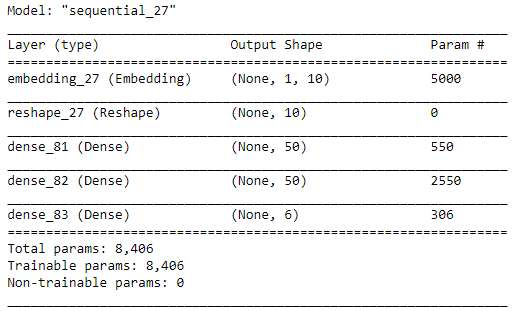
Now let’s run the training using the steps explained in the previous chapter:

 You can notice that this process is fairly similar to the training process we explored in the previous chapter for standard Q-Learning.

Conclusion

In this article we explored Deep Q-Learning. This is the first type of reinforcement learning that utilize neural networks. By this we solved scaling problem we had with standard Q-Learning and paved the way for more complex systems.

Thank you for reading!