In the past couple of years, convolutional neural networks became one of the most used deep learning concepts. They are used in a variety of industries for object detection, pose estimation, and image classification. For example, in healthcare, they are heavily used in radiology to detect diseases in mammograms and X-ray images.

One concept of these architectures, that is often overlooked in the literature is the concept of the receptive field. In essence, all state-of-the architectures use this concept to build their ideas around it. That is why in this article, we explore what are receptive fields, how they are defined, and how we can calculate their size.

To understand the concepts in this article, we assume that you are familiar with convolutional operations, pooling operations, and other basic Convolutional Neural Networks principles. If you need to learn more about these concepts make sure to check out our Ultimate Guide to Machine Learning with Python.

In this article we cover:

1. What are Receptive Fields in Convolutional Neural Networks?

2. Math of the Receptive Fields in CNN

3. Python Implementation

1. What are Receptive Fields in Convolutional Neural Networks?

As a quick reminder, Convolutional Neural Networks use kernels (or filters) to detect features in images. This is done by using convolution operations over the image. Every kernel “looks” at a certain part of the input image, perform multiplications and then moves by a defined number of pixels (stride). This area in the input space that a particular CNN’s kernel is looking at is called Receptive Field.

Convolution Process

Receptive fields are defined by the center and the size. The center of the receptive field is very important since it decides the importance of the pixel. If the pixel is located closer to the center its importance in that particular computation is higher. This means that the CNN feature focuses more on the central pixel of the receptive field.

Convolutional Neural Network updates its kernel biases based on this, which is why the receptive field is such an important concept. Since modern CNNs are deep, meaning stack multiple convolutional layers, the receptive field for each layer is different. If the layer is deeper in the architecture, its receptive field will be larger because its input space is feature maps from previous layers, ie. already downsampled input image.

Let’s observe the following example. An input image is 5×5 and we use two convolutional layers. Both layers use 3×3 kernels, 2×2 stride and 1×1 padding:

The first layer creates a feature map that is 3×3. Its receptive field has the same size. The second layer performs convolution on the output of that feature map and creates 2×2 feature map. Ok, that is cool, but what is the receptive field of the second layer? Remember, the receptive field is the space in the input image, not in the feature map. Here it is:

Receptive Field of the Second Layer

It is interesting to observe it like this too:

Receptive Fields on the first and second layers (left) and Centers of receptive fields of the first and second layer (right) Source

In the right-side images, we can observe centers of receptive fields. Note how stride accumulates after each layer and how centers of the first layer are closer to each other than the strides of the second layer.

2. Math of the Receptive Fields in CNN

Now, we have some intuition about what receptive fields are and how the depth of the architecture changes it. Let’s go a bit deeper and get the math behind it. The first step when it comes to this calculation is getting the size of the output feature map for each layer. This is calculated by the formula:

where ni  is the number of the output features for the layer i, ni-1 is the number of the input features for the layer i, p is the padding size the layer i, k is the kernel size of the layer i and s is the stride of the layer i. Then we need to calculate the jump. The jump, in general, represents the cumulative stride. We can get it by multiplying strides of all layers that came before the layer that we are investigating. We can use this formula:

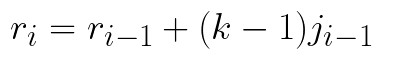
where ji-1 is the jump of the previous layer. Finally, using previous values, we can calculate size of the receptive field, using this formula:

The more general form of the formula above that is used for calculating the receptive field of certain layer looks like this:

As we mentioned, the receptive field is defined by the center and the size. So here is the formula for calculating center of the receptive field for the given layer:

At this moment you might wonder what would be the values for the input image since we don’t have the previous layer for it. For the input image we use these values:

• n = image size
• r = 1
• j = 1
• start = 0.5

Let’s apply these formulas to our example from before. Layer 0 is the input image and its dimensions are 5×5 which means n0 is 5. By the default r0, j0 and start0 are 1, 1, and 0.5, respectively. When we apply previous functions to the second layer we get values n1 = 2, r1 = 7, j2=4, start1 = 0.5.

Note that in these examples, in order to simplify, we are assuming the CNN architecture is symmetric, and the input image is square.

3. Implementation with Python

Ok, let’s implement these calculations in Python. Let’s say that we want to have use a dictionary to describe CNN architecture. For example, AlexNet would look like something like this:

Key is the name of the layer and the value is the array consisting of kernel size, stride and padding respectively. This means that layer conv2 has 5×5 kernel, 1×1 striding and 2×2 padding. Next, we implement ReceptiveFieldCalculator class like this:

This class has three methods:

• calculate – a public method that orchestrates calculation and printing of output feature map size, jump, receptive image size and the center.
• _print_layer_info – helper method used for printing out information
• _calculate_layer_info – helper method used for calculations

3.1 How to use it?

Here is how we use it:

Conclusion

In this article, we explored interesting and sometimes overlooked concepts of receptive fields. We had a chance to get the intuition and math behind it and implement one version of a receptive field calculator using Python.

Thank you for reading!