Machine Learning, Neural Networks and Artificial intelligence are big buzzwords of the decade. It is not surprising that today these fields are expanding pretty quickly and are used to solve a vast amount of problems. We are witnesses of the new golden period of these technologies. However, today we are merely innovating. Majority of the concepts used in these fields were invented 50 or more years ago. In fact, all ideas are based heavily on math.

This is the most troubling part for the people who are trying to get into the field. The most usual question that I get on the meetups and conferences is “How much math should I know?”. Those were all the people with software development background trying to get into the data science world. Actually, this was the question that I asked myself long ago when I started my journey through this universe. One of the big challenges was blowing off dust from old college books and trying to remember stuff that was forgotten during the years in the software development industry.

Concepts that were so useful and that helped me work on high-quality software couldn’t help me, which was exciting and scary. So, I had to go to the basics and re-figure some things out. In this article, I will try to cover as much ground as possible. There will be stuff left out, simply because on this topic I could easily write a book about (well, not easily, per se, but you get my point). Please, feel free to explore these topics further, and gather as much knowledge as possible.

While some people will argue that even this much math is too much, in my humble opinion, knowing this bare minimum will help you understand concepts of machine learning and AI in more depth, which in turn will give you the ability to easily switch programming languages, technology stacks, and frameworks. There are three big areas that we will explore: Linear Algebra, Calculus and Probability. In this first article of the series, we will explore the basic concepts of Linear Algebra that you should know about.

Basic Terms

In general, linear algebra revolves around several types of basic mathematical terms. When we are talking about this branch of math we are using terms: scalar, vector, matrix, and tensor. They are very important for machine learning because using them we can abstract data and models. This means that for example, every record in a dataset can be represented as a vector in a multi-dimensional space and parameters of neural networks are abstracted as matrices. More on this later. Every one of these mathematical objects has its specifics, so let’s check them one by one.

Scalar is just one simple number, in contrast to the vectors and matrices. They are defined as elements of the field that are used to describe vector space. Multiple scalars create a vector. They can be a different type of number, and when we describe them we usually mention what kind of number they are (real, natural, etc.). They have lowercase italic names like this:

Vector is essentially an ordered array of scalars, meaning it is an ordered array of numbers. We are considering them as points in space, where each element defining coordinate on a certain axis. Collection of vectors create so-called vector space. They can be added together, multiplied, or scaled (multiplied by scalar). They have lowercase bold names, with each element having an index:

Matrix is a two-dimensional array of scalars with an uppercase bold name. For example, if we talk about a real-valued matrix with m rows and n columns, we will define it like this:

Since we are having two dimensions, elements of the matrix have two indexes:

Matrices can be added or subtracted element-wise, only if they have the same number of rows and columns. Two matrices can be multiplied only when the number of the columns of the first matrix is equal to the number of the rows of the second one. For example, you can multiply matrix A with dimensions m, n with matrix B with dimensions n, p. As a result, you will get a matrix C with dimensions m, p. The product, also called dot product, is defined as:

It is important to note that dot product is distributive and associative:

However, sometimes we need to multiply matrices element-wise. That operation is alternately called the Hadamard product and is denoted as A
∘ B. Same as a vector, any matrix can be multiplied with a scalar element-wise. Another interesting fact is that a product of matrix and vector is a vector:

Tensor is a multidimensional array of numbers. Basically, it has more than two dimensions, so it can be visualized as a multidimensional grid of numbers. In essence, matrices are also tensors with two dimensions. That is why the same rules apply to these objects. Tensors are popularised through Machine Learning frameworks like TensorFlow.

Operations

Matrices have several operations that we need to explore and learn if we want to understand some functions of machine learning, deep learning and artificial intelligence applications. One of those operations is the transpose operation. The result of this operation is the so-called transpose matrix. Essentially that is a mirror image of the matrix across the main diagonal line. This line starts in the upper left corner of the matrix and goes down and to the right. Transpose matrix of the matrix A is denoted as
A^T (alternatively: A′, A^tr, ^tA or A^t). Another way to get the transpose matrix is to write the rows of A as the columns of A^T and write the columns of A as the rows of A^T.

Another interesting term when it comes to matrices is the identity matrix. This is a matrix that doesn’t change any value in a vector when it is multiplied with it. Basically, it has values 1 along the main diagonal, while other values are zero. It is defined like this:

Similar to that inverse matrix is defined like this:

When we multiply matrix A with its inverse matrix A^-1 we get an identity matrix. You can observe this kind of matrix like a reciprocal number. Meaning, since the reciprocal number of a is 1/a, that means that number*reciprocal number = 1. Here is the same situation, only we are using matrices. This process is not defined for non-squared matrices. If we are having this kind of matrix we can apply Moore-Penrose pseudoinverse. In its practical form, it is defined as:

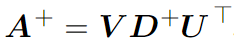
where U, D and V are the singular value decomposition of A. The is pseudoinverse D⁺ of a matrix D is created by taking the reciprocal value of its elements and then taking the transpose of the resulting matrix. However, be careful with the concept of inverse matrix A^-1, because it is more used in theory than in practice, especially when it comes to a software application. This is due to the fact that it can only be represented with limited precision on a computer.

Before we proceed, let’s just observe the diagonal matrix. This matrix is similar to the identity matrix. This matrix is having zero values everywhere except on the main diagonal. In contrast to the identity matrix, the diagonal matrix has values different than 1. We can say that the identity matrix is one type of diagonal matrix. These matrixes are exceptionally useful for some algorithms.

In some situations, we want to map the matrix into a scalar. This is done by using determinant – det(A) or |A|. This operation is applicable only to square matrices. In the case of a 2×2 matrix the determinant is defined like this:

Finally, let’s mention linear dependency. Set of vectors is linearly dependent if at least one vector can be represented as a combination of other vectors from the set. Otherwise, this set is linearly independent. Basically, vectors x and y are linearly independent if only values for scalars a and b satisfying ax+by=0 are a = b = 0.

Norms

In order to properly work with vectors, we sometimes need to know the size of the vector. This is usually done using functions that are called norms – Lⁿ. The letter n is defining the number of dimensions in which our vector exists. Depending on how many of the dimensions our vector space has this norm function is different. The most well-known norm is the norm in two-dimensional space – L² norm or Euclidian norm. Basically, it represents Euclidean distance from the origin of the vector to the point in space that is described with that vector. When we generalize this to more dimension we get global norm function:

In general, the norm is any function that follows these rules:

1. f(x + y) ≤ f(x) + f(yv) (satisfying the triangle inequality).
2. f(ax) = |a| f(x) (being absolutely scalable).
3. If f(x) = 0 then x = 0 (being positive definite)

Often when we are building AI application it is important to discriminate between elements which have value 0 and elements that are having a value close to 0. For this, we use the L¹ norm. This function is simple and keeps the same growth rate in all points of a vector space. Basically, if any element of the vector x moves from 0 to a this function increases by a. The first norm is defined like this:

As we mentioned previously, in deep learning, we abstract parameters of the neural networks as matrices. This means that sometimes we need the size of the matrix. This is obtained using the Frobenius norm:

Conclusion

In this article, we explored some major topics of the linear algebra that you need to know in order to understand what is going on in machine learning, deep learning and artificial intelligence applications. However, these are just starting points and I encourage you to explore these topics in more depth.

Thank you for reading!

---

Read more posts from the author at Rubik’s Code.

---