Getting into machine learning, deep learning and artificial intelligence is not easy. These are all very cool and interesting topics, and they are being hyped lately, but like with software development, it is not for everybody. Some would say that if you are having a software development background, you are having a certain advantage. While this is true to an extent, this attitude can be a double-edged sword. Especially when it comes to math which supports all important concepts from these fields.

In fact, the most usual question that I get on the meetups and conferences from the software developers is “How much math should I know?”. This was the same question that I asked myself long ago when I started my journey into the data science world. One of the big challenges was blowing off dust from old college books and trying to remember stuff that was forgotten during the years in the software development industry.

The problem is that education and ways of thinking of us software developers usually revolve about discrete mathematics, while some topics that are utilized in AI are not used that much. The idea is to cover these big areas: Linear Algebra, Calculus and Probability in a series of articles. In the previous article, we started a journey into these topics with linear algebra. Of course, these articles can not replace prerequisite classes. There will be things that are left out, simply because on each of these topics we could easily write a book about (well, not easily, per se, but you get my point). Please, feel free to explore them further, and gather as much knowledge as possible.

While some people will argue that even this much math is too much, in my humble opinion, knowing this bare minimum will help you understand concepts of machine learning and AI in more depth, which in turn will give you the ability to easily switch programming languages, technology stacks, and frameworks. In this article, we will explore the basic concepts of Probability that you should know.

Basic Terms

It might be a little bit weird to work with probabilities in computer science since most of the branches of deal with deterministic and certain entities. However, when we are talking about artificial intelligence or data science in general, uncertainty and stochasticity can appear in many forms. Data is, of course, the main source of uncertainty, but a model can be a source as well. Probability theory provides tools for modeling and dealing with uncertainty. We use this theory for analyzing frequencies of occurrence of events.

Probability can be defined as the likelihood or chance of an event occurring. Essentially it is a number between 0 and 1, where 0 indicates impossibility and 1 indicates certainty of occurrence of an event. The probability of an event A is written as P(A) or p(A). Formally we can say that if P(A) = 1, A occurs almost surely and A occurs almost never if P(A) = 0. Using this we can define P(A^c), which is called the complement of the event, and it means that A is not occurring. It has value P(A^c) = 1 – P(A).

When we are talking about the probability of multiple events and the relationship of those probabilities we use the term joint probability. Essentially is a statistical measure that represents the chance of two events occurring together. If those events are independent this is how we define it:

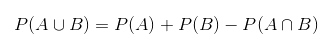
However, if those events are mutually exclusive, then we need to extend these calculations like this:

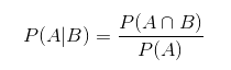
Finally, let’s define some terms that are very useful when it comes it comes to probability calculations. Often we are interested in the probability of some event A, given that another event B has happened. This is a conditional probability:

Another interesting thing is that joint probability over many random variables may be split into conditional distributions over one variable. This occurrence is called as the chain rule (product rule) of probability:

In the end, let’s mention a simple but crucial Bayes’ rule. It describes the probability of an event, based on prior knowledge of conditions or other events that are related to the event. It is defined like this:

Or in it’s normalized version:

In the literature, P(A) is often called the prior, P(A|B) – the posterior, and P(B|A) – likelihood. When we are talking about machine learning, deep learning or artificial intelligence, we use Bayes’ rule to update parameters of our model (i.e. wights of the neural network’s connections).

Random Variables and Probability Distribution

A random variable is defined as a variable which can take different values randomly. Or more formally, it is defined as a function which transfers results of some changeable process into numerical values. Mathematically, they can be defined as:

where Ω is a set of possible outcomes, and E is some measurable space. However, random variable on its own just a placeholder, meaning it just holds possible states for some process. In order for it to make sense, it has to be paired with some probability distribution, which will say how likely are some of those states are. Random variables can be discrete or continuous and based on that there are few ways to describe probability distribution.

Discrete random variables have a finite (or countably infinite) number of states. We can observe them as categorical variables or enumerations. The probability distribution over this type of random variables is described using probability mass function – PMF. This function gives the probability that a discrete random variable is equal to some value. Suppose that X:
Ω → [0, 1], is a discrete random variable that maps set of possible outcomes Ω to space with values 0 and 1. Than probability mass function p is defined as:

On the other hand, continuous random variables have values from the set of real numbers. This means that they have an infinite number of states.
The probability distribution over this type of random variables is described using probability density function – PDF. This function must satisfy certain conditions. First, the domain of p must be the set of all possible states of x. Apart from that, this function must have a value bigger than 1 for all values of x. Finally, it has to satisfy the condition:

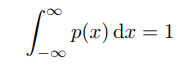
The trick with this function is that it doesn’t give the probability of state directly, but it gives the probability of landing inside an infinitely small region of that state. This is due to the fact that the likelihood of a continuous random variable taking any particular state is 0 because there is an infinite number of possible states. The probability that x lies in the interval [a, b] is given by:

Expectation, Variance and Covariance

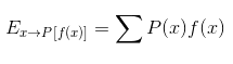
In probability, expectation (expected value) is defined as an average value of repetition of some event. More formally, the expected value of some function f(x) over probability distribution P(x) is the mean value of f when x is taken from P. For discrete random variables we define it like this:

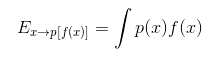
While for continuous random variables we define it like this:

We may say that this value provides a measure of the “center” of a distribution. However, we are also interested in what the “spread” is around that center. Meaning we want to know how values of a function f(x) of a random variable x vary as we take different values from its probability distribution P(x). This is called variance and it represents the average squared deviation of the values of f(x) from the mean of f(x) :

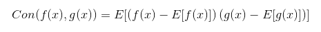
The square root of this value is called standard deviation. Using this, we can define covariance. Essentially it is a measure of the linear relationship between two random variables. It gives us sense of how much two values are linearly related. Mathematically it is described like this:

Conclusion

In this article, we explored some major topics of the probability that you need to know in order to understand what is going on in machine learning, deep learning and artificial intelligence applications. However, these are just starting points and I encourage you to explore these topics in more depth.

Thank you for reading!

---

Read more posts from the author at Rubik’s Code.

---