If you followed previous blog posts on this site, you noticed that we covered a range of math topics that you should know in order to understand concepts behind machine learning, deep learning and artificial intelligence. So far, we went through linear algebra and probability theory. The trend continues in this article, where we will explore calculus and optimization. One might ask “Why are we doing this and what is the benefit of it?”.

Well, even though machine learning and artificial intelligence are quite buzzwords these days, they all lay on concepts that were laid down 50 years ago. These concepts are heavily based on math. If you come from the software development world, some of these topics are not used as often in the industry, so we tend to forget them even if we have some formal/informal education. We mostly deal with discrete mathematics in software development, which is not always the case when we are working on AI applications.

Apart from that, one of the most frequent question on data science meetups and conferences is “How much math should I know in order to get into the field?”. This question comes from people with software development background. So, one of the challenges of getting into the field is certainly blowing off dust from old college books, going back to basics and re-learning some stuff.

While some people can (and will) argue you can get away with not knowing these topics, in my humble opinion, learning this bare minimum will help you understand mentioned AI concepts in more depth. That way you will be able to easily switch technology stacks, frameworks and programming languages.

Note that there are be things that are left out in all these math articles. On each of these, we could easily write a book about (well, not easily, per se, but you get my point). Please, feel free to explore them further, and gather as much knowledge as possible. Ok, let’s check out Calculus and Optimization.

Basic Terms

Machine learning and deep learning applications usually deal with something that is called the cost function, objective function or loss function. This function, in general, represents how good or bad model that we created fits data that we work with. Meaning, it is giving us some sort of scalar value that is telling us how much our model is off. This value is used to optimize the parameters of the model and get better results on the next samples from the training set. For example, you can check how the backpropagation algorithm updates weights in neural networks based on this concept.

In order for our model to fit data the best way possible, we would have to to find the global minimum of the cost function. However, finding that global minimum and changing all those parameters is usually very costly and time-consuming. That is why we are using iterative optimization techniques like gradient descent. Ok, I really went too fast too soon. Let’s first see what is global minimum, or even better let’s see what are the extrema of some function and what are tools we are using for finding them.

Essentially, optimization is all about finding extrema of some function, or to be more precise, finding the minima and maxima. Also, when we are doing some sort of optimization, we always need to consider a set of values for an independent variable over which we are doing it. This set of values is often called the feasible set or feasible region. Mathematically speaking it is always a subset of real numbers set X ⊆ R. If the feasible region is the same as the domain of the function, e.g. if X represents the complete set of possible values of the independent variable, the optimization problem is unconstrained. Otherwise, it is constrained and much harder to solve.

Ok, but what are minima and maxima? We are defining two types of minima and maxima – local and global. A local minimum of function f in X is defined as f(x) ≤ f(y) for every y in the neighborhood T around x, where T ⊆ X. Furthermore, if f(x) ≤ f(y) for every y ∈ X, x is a global minimum of the function f. Similarly, a local maximum of function f in X is defined as f(x) ≥ f(y) for every y in the neighborhood T around x, where T ⊆ X. If f(x) ≤ f(y) for every y ∈ X, x is a global maximum of the function f.

There can be only one global minimum (resp. maximum) or multiple global minima (resp. maxima) of the function. It is also possible for there to be local minima that are not globally optimal. In the context of machine learning and deep learning, we usually optimize functions that may have many local minima. At this moment you might wonder how we can find these values in some functions? For finding minima and maxima we are using derivatives.

Derivative

Let’s consider a function y=f(x), where x∈ R and y∈ R. The first derivative of this function is defined as f'(x) or as:

In its essence, derivative gives us the slope at the point x. Meaning that it describes how a small change in the input x will affect output y. Mathematically we can say it like this:

If f'(x)=0 this means that there is no slope, meaning small changes in the x will not change the value of y. This means we have hit stationary point at point x. Minimum and maximum are both types of stationary points. The third type of stationary point is so-called saddle point. It has slope zero but it is no minimum nor maximum.

So far we considered only function with one input. However, when we are talking about functions with multiple inputs we use the concept of partial derivative:

This derivative describes how output changes at point x if only variable xi changes. As you know, when we are working on machine learning, deep learning or AI applications, a single sample of data is usually represented with vector. That is why partial derivative is exceptionally useful.

Another term we should cover when we are talking about derivatives is directional derivative. This derivative represents the slope in the direction d (unit vector). In a nutshell, it is a derivative of the function f(x+ad)
with respect to a, evaluated at a= 0.

Gradient Descent

The most important concepts from calculus in the context of AI are gradient and gradient descent. We already mentioned that we are using gradient descent for getting to the minima of some function, but we haven’t explained what does that technique considers. Loosely speaking gradient groups all partial derivatives, the gradient is just the vector containing all the partial derivatives. In essence, it generalizes derivatives to scalar functions of several variables.

Why the gradient is so important? Well, just like the first derivative of a function with one variable equals to zero in stationary points, the same goes for gradient for the functions with multiple variables. Another cool thing about gradient ∇f(x) is that it points in the steepest ascent from x. On the other hand, −∇f(x) points in the direction of steepest descent from x. This is heavily utilized by mentioned gradient descent technique. This technique is used to iteratively find a minimum of a function.

It starts from one point x, in which by calculating gradient it gets the information about where the minimum is because we get the steepest descent in x. Then it goes to the new point calculated by the formula:

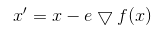
where e is called the learning rate. Then the whole process is repeated in the point x’.

The Jacobian & The Hessian

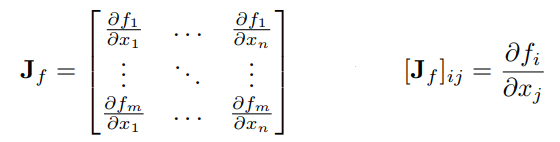
What we learned so far is that the gradient of the function equals to zero in stationary points. However, this information can be misleading, meaning that we have found a saddle point, not minimum or maximum. For this, we use the second derivative. Before we continue with other conditions for local minimum, let’s introduce matrices of derivatives – the Jacobian and the Hessian. As you already know, we are dealing with a lot of matrices in machine learning, deep learning and AI. That is why we need to extend our notion of derivatives. The Jacobian is the matrix of first derivatives:

Similarly, the Hessian is the matrix of the second derivatives:

The Hessian is expensive to calculate, but it is extremely useful. It is used in optimization techniques such as Newton’s method.

Using this, we can define conditions for the local minimum: If function f is twice continuously differentiable with ∇²f positive semi-definite in a neighborhood of x, and that ∇f(x) = 0. Then x is a local minimum of f.

Conclusion

Calculus and optimization are huge topics, that are not always intuitive and require a lot of practice. In this article, we tried to extract important concepts that should be investigated in more depth in order to understand how machine learning, deep learning and artificial intelligence algorithms work. Here we just scratched the surface of optimization techniques that are used in such algorithms. However, it is a good starting point from which you can build on.

Thank you for reading!

---

Read more posts from the author at Rubik’s Code.

---