

It is always fun and educational to read deep learning scientific papers. Especially if it is in the area of the current project that you are working on. However, often these papers contain architectures and solutions that are hard to train. Especially if you want to try out, let’s say, some of the winners of ImageNet Large Scale Visual Recognition (ILSCVR) competition. I can remember reading about VGG16 and thinking “That is all cool, but my GPU is going to die”. In order to make our lives easier, TensorFlow 2 provided a number of pre-trained models, that you can quickly utilize. In this article, we are going to find out how you can do that with some of the famous Convolutional Neural Network architectures.
At this moment one might wander “What are pre-trained models?”. Essentially, a pre-trained model is a saved network that was previously trained on a some large dataset, for example on ImageNet dataset. They can be found in tensorflow.keras.applications module. There are two ways in which you can use those. You can use it as out of the box solution and or you can use it with transfer learning. Since, large datasets are usually used for some global solution you can customize pre-trained model and specialize it for certain problem. This way you can utilize some of the most famous neural networks without loosing too much time and resources on training. Additionally, you can fine tune these models, by modifying behavior of the chosen layers. This will be covered in the future articles.
Architectures

In this article, we use three pre-trained models to solve classification example: VGG16, GoogLeNet (Inception) and ResNet. Each of these architectures was winner of ILSCVR competition. VGG16 had the best results together with GoogLeNet in 2014 and ResNet won in 2015. These models are part of the TensorFlow 2, i.e. tensorflow.keras.applications module. Let’s dig a little deeper about each of these architectures.
VGG16 is the first architecture we consider. It is a large convolutional neural network proposed by K. Simonyan and A. Zisserman in the paper “Very Deep Convolutional Networks for Large-Scale Image Recognition”. this network achieves 92.7% top-5 test accuracy in ImageNet dataset. However, it was trained for weeks. Here is high-level overview of the model:

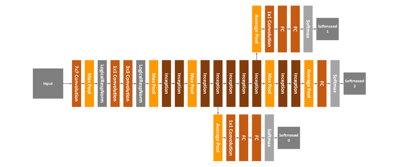
GoogLeNet is also called Inception. This is because it utilizes two concepts: 1×1 Convolution and Inception Module. The first concept, 1×1 Convolution is used for as a dimension reduction module. By reducing number of dimensions, number of computations also goes down, which means that depth and width of the network can be increased. Instead of using fixed size for each convolution layer, GoogLeNet uses Inception Module:

As you can see 1×1 convolution layer, 3×3 convolution layer, 5×5 convolution layer, and 3×3 max pooling layer perform their operations together and than their results are stack together again at output. GoogLeNet has 22 layer in total, and it looks something like this:
Residual Networks or ResNet are the final architecture we are going to use in this article. The problem that previous architecture have is that they are very deep. They have a lot of layers and because of that they are hard to train (vanishing gradient). So, ResNet addressed that problem with so-called “identity shortcut connection”, or residual blocks:

In essence, ResNet follows VGG’s 3×3 convolutional layer design, where each convolutional layer is followed by a batch normalization layer and ReLU activation function. The difference is however that we before the final ReLu, ResNet injects input. One of the variations is that, input value is passes through the 1×1 convolution layer.
Dataset

In this article, we use “Cats vs Dogs” dataset. This dataset contains 23,262 images of cats and dogs.
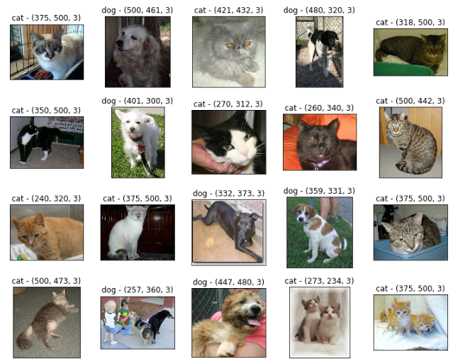
You may notice that images are not normalized and that they have different shapes. The cool thing is that it is available as a part of TensorFlow Datasets. So, make sure that you have installed TensorFlow Dataset in your environment:
pip install tensorflow-dataset
Unlike other datasets from the library this dataset is not divided into train and test data so we need to perform the split ourselves. You can find more information about the dataset here.
Implementation

This implementation is split into several parts. First we implement class that is in charge of loading data and preparing it. Then we import pre-trained models and build a class that will modify it’s top layers. Finally we run the training process and evaluation process. Before everything, of course, we have to import some libraries and define some global constant:
| import numpy as np | |
| import matplotlib.pyplot as plt | |
| import tensorflow as tf | |
| import tensorflow_datasets as tfds | |
| IMG_SIZE = 160 | |
| BATCH_SIZE = 32 | |
| SHUFFLE_SIZE = 1000 | |
| IMG_SHAPE = (IMG_SIZE, IMG_SIZE, 3) |
All right, let’s dive into the implementation!
Data Loader
This class is in charge of loading the data and preparing it for processing. Here is what it looks like:
| class DataLoader(object): | |
| def __init__(self, image_size, batch_size): | |
| self.image_size = image_size | |
| self.batch_size = batch_size | |
| # 80% train data, 10% validation data, 10% test data | |
| split_weights = (8, 1, 1) | |
| splits = tfds.Split.TRAIN.subsplit(weighted=split_weights) | |
| (self.train_data_raw, self.validation_data_raw, self.test_data_raw), self.metadata = tfds.load( | |
| 'cats_vs_dogs', split=list(splits), | |
| with_info=True, as_supervised=True) | |
| # Get the number of train examples | |
| self.num_train_examples = self.metadata.splits['train'].num_examples*80/100 | |
| self.get_label_name = self.metadata.features['label'].int2str | |
| # Pre-process data | |
| self._prepare_data() | |
| self._prepare_batches() | |
| # Resize all images to image_size x image_size | |
| def _prepare_data(self): | |
| self.train_data = self.train_data_raw.map(self._resize_sample) | |
| self.validation_data = self.validation_data_raw.map(self._resize_sample) | |
| self.test_data = self.test_data_raw.map(self._resize_sample) | |
| # Resize one image to image_size x image_size | |
| def _resize_sample(self, image, label): | |
| image = tf.cast(image, tf.float32) | |
| image = (image/127.5) – 1 | |
| image = tf.image.resize(image, (self.image_size, self.image_size)) | |
| return image, label | |
| def _prepare_batches(self): | |
| self.train_batches = self.train_data.shuffle(1000).batch(self.batch_size) | |
| self.validation_batches = self.validation_data.batch(self.batch_size) | |
| self.test_batches = self.test_data.batch(self.batch_size) | |
| # Get defined number of not processed images | |
| def get_random_raw_images(self, num_of_images): | |
| random_train_raw_data = self.train_data_raw.shuffle(1000) | |
| return random_train_raw_data.take(num_of_images) |
There is a lot going on in this class. It has several methods of which one is “public”:
- _prepare_data – Internal method used to resize and normalize images from dataset. Utilized from constructor.
- _resize_sample – Internal method used for resizing single image.
- _prepare_batches – Internal method used to create batches from images. Creates train_batches, validation_batches and test_batches that are used for training and evaluation process.
- get_random_raw_images – Method used to get certain number of random images from raw, non processed data.
However, majority of things happen in the constructor of the class. Let’s take a closer look.
| def __init__(self, image_size, batch_size): | |
| self.image_size = image_size | |
| self.batch_size = batch_size | |
| # 80% train data, 10% validation data, 10% test data | |
| split_weights = (8, 1, 1) | |
| splits = tfds.Split.TRAIN.subsplit(weighted=split_weights) | |
| (self.train_data_raw, self.validation_data_raw, self.test_data_raw), self.metadata = tfds.load( | |
| 'cats_vs_dogs', split=list(splits), | |
| with_info=True, as_supervised=True) | |
| # Get the number of train examples | |
| self.num_train_examples = self.metadata.splits['train'].num_examples*80/100 | |
| self.get_label_name = self.metadata.features['label'].int2str | |
| # Pre-process data | |
| self._prepare_data() | |
| self._prepare_batches() |
First we define image and batch size that are injected through parameters. Then, since dataset is not already split into training and testing data, we split data using split weights. This is really a cool feature that TensorFlow Dataset introduced, because we stay within TensorFlow ecosystem and we don’t have to involve other libraries like Pandas or SciKit Learn. Once we performed data split we calculate the number of the training samples and call helper function that prepares data for training. All we need to do after this is to instantiate an object of this class and have fun with loaded data:
| data_loader = DataLoader(IMG_SIZE, BATCH_SIZE) | |
| plt.figure(figsize=(10, 8)) | |
| i = 0 | |
| for img, label in data_loader.get_random_raw_images(20): | |
| plt.subplot(4, 5, i+1) | |
| plt.imshow(img) | |
| plt.title("{} – {}".format(data_loader.get_label_name(label), img.shape)) | |
| plt.xticks([]) | |
| plt.yticks([]) | |
| i += 1 | |
| plt.tight_layout() | |
| plt.show() |
Here is the output:
Base Models & Wrapper
Next thing on our list is loading of the pre-trained models. As we already mentioned these models are located in tensorflow.kearas.applications. Loading them is pretty straight forward:
| vgg16_base = tf.keras.applications.VGG16(input_shape=IMG_SHAPE, include_top=False, weights='imagenet') | |
| googlenet_base = tf.keras.applications.InceptionV3(input_shape=IMG_SHAPE, include_top=False, weights='imagenet') | |
| resnet_base = tf.keras.applications.ResNet101V2(input_shape=IMG_SHAPE, include_top=False, weights='imagenet') |
That is how we created based models of the three architectures of interest. Notice that for every model include_top parameter is defined as False. This means that these models are used for feature extraction. Once we have them, we need to modify top layers of these models so they are applicable to our concrete problem. We do that using Wrapper class. This class accepts injected pre-trained model and adds one Global Average Polling Layer and one Dense layer. Essentially, the final Dense layer is used for our binary classification (car or dog). Wrapper class puts all these things together into one model:
| class Wrapper(tf.keras.Model): | |
| def __init__(self, base_model): | |
| super(Wrapper, self).__init__() | |
| self.base_model = base_model | |
| self.average_pooling_layer = tf.keras.layers.GlobalAveragePooling2D() | |
| self.output_layer = tf.keras.layers.Dense(1) | |
| def call(self, inputs): | |
| x = self.base_model(inputs) | |
| x = self.average_pooling_layer(x) | |
| output = self.output_layer(x) | |
| return output |
Then we can create real models for classification Cats vs Dogs dataset and compile those models:
| base_learning_rate = 0.0001 | |
| vgg16_base.trainable = False | |
| vgg16 = Wrapper(vgg16_base) | |
| vgg16.compile(optimizer=tf.keras.optimizers.RMSprop(lr=base_learning_rate), | |
| loss='binary_crossentropy', | |
| metrics=['accuracy']) | |
| googlenet_base.trainable = False | |
| googlenet = Wrapper(googlenet_base) | |
| googlenet.compile(optimizer=tf.keras.optimizers.RMSprop(lr=base_learning_rate), | |
| loss='binary_crossentropy', | |
| metrics=['accuracy']) | |
| resnet_base.trainable = False | |
| resnet = Wrapper(resnet_base) | |
| resnet.compile(optimizer=tf.keras.optimizers.RMSprop(lr=base_learning_rate), | |
| loss='binary_crossentropy', | |
| metrics=['accuracy']) |
Note that we marked that base models are not trainable. This means that during the training process we will train only top layers that we have added and the weights on the lower layers will not change.
Training
Before we get into the whole training process, let’s reflect on the fact that in principle biggest part of these models is already trained. So, what we can do is perform evaluation process and see where we land:
| steps_per_epoch = round(data_loader.num_train_examples)//BATCH_SIZE | |
| validation_steps = 20 | |
| loss1, accuracy1 = vgg16.evaluate(data_loader.validation_batches, steps = 20) | |
| loss2, accuracy2 = googlenet.evaluate(data_loader.validation_batches, steps = 20) | |
| loss3, accuracy3 = resnet.evaluate(data_loader.validation_batches, steps = 20) | |
| print("——–VGG16———") | |
| print("Initial loss: {:.2f}".format(loss1)) | |
| print("Initial accuracy: {:.2f}".format(accuracy1)) | |
| print("—————————") | |
| print("——–GoogLeNet———") | |
| print("Initial loss: {:.2f}".format(loss2)) | |
| print("Initial accuracy: {:.2f}".format(accuracy2)) | |
| print("—————————") | |
| print("——–ResNet———") | |
| print("Initial loss: {:.2f}".format(loss3)) | |
| print("Initial accuracy: {:.2f}".format(accuracy3)) | |
| print("—————————") |
It is interesting that without prior training of any of these models, we get ok-ish results (50% accuracy):
———VGG16———
Initial loss: 5.30
Initial accuracy: 0.51
—————————-
——GoogLeNet—–
Initial loss: 7.21
Initial accuracy: 0.51
—————————-
——–ResNet———
Initial loss: 6.01
Initial accuracy: 0.51
—————————-
Starting with 50% accuracy is not bad thing at all. So, let’s run training process and see are we getting any better. First we train VGG16:
| history = vgg16.fit(data_loader.train_batches, | |
| epochs=10, | |
| validation_data=data_loader.validation_batches) |
The history looks something like this:

Then we train GoogLeNet:
| history = googlenet.fit(data_loader.train_batches, | |
| epochs=10, | |
| validation_data=data_loader.validation_batches) |
History of this training process looks like this:

Finally we train ResNet:
| history = resnet.fit(data_loader.train_batches, | |
| epochs=10, | |
| validation_data=data_loader.validation_batches) |
And here is the history of that process:

Training of these three models lasted just couple of hours, instead for weeks, thanks to the fact that we trained just top layers and not the whole network.
Evaluation
We saw that in the begining, without any training we got around 50% of accuracy. Let’s see what is the situation after the training:
| loss1, accuracy1 = vgg16.evaluate(data_loader.test_batches, steps = 20) | |
| loss2, accuracy2 = googlenet.evaluate(data_loader.test_batches, steps = 20) | |
| loss3, accuracy3 = resnet.evaluate(data_loader.test_batches, steps = 20) | |
| print("——–VGG16———") | |
| print("Loss: {:.2f}".format(loss1)) | |
| print("Accuracy: {:.2f}".format(accuracy1)) | |
| print("—————————") | |
| print("——–GoogLeNet———") | |
| print("Loss: {:.2f}".format(loss2)) | |
| print("Accuracy: {:.2f}".format(accuracy2)) | |
| print("—————————") | |
| print("——–ResNet———") | |
| print("Loss: {:.2f}".format(loss3)) | |
| print("Accuracy: {:.2f}".format(accuracy3)) | |
| print("—————————") |
Here is the output:
——–VGG16———
Loss: 0.25
Accuracy: 0.93
—————————
——–GoogLeNet———
Loss: 0.54
Accuracy: 0.95
—————————
——–ResNet———
Loss: 0.40
Accuracy: 0.97
—————————
We can see that all three models are having really good results, with ResNet being in the front with 97% accuracy.
Conclusion
In this article, we demonstrated how to perform transfer learning with TensorFlow. We created a playground in which we can try out different pre- trained architectures on the data and get good results after just a matter of hours. In our example, we worked with three famous convolutional architectures and quickly modified them for specific problem. In next article, we will fine tune these models and check if we can get even better results.
Thank you for reading!
Read more posts from the author at Rubik’s Code.


Thank you for this very well written and informative article! I’m looking to do exactly this during the coming week, and this is a great head start. I just have three questions:
1) What does super(Wrapper, self).__init__() do?
2) In general, what do you think is the best resource for tf documentation? The tensorflow documentation itself is really sparse, just listing available methods with no explanation.
3) How can the validation error be lower than the training error for Googlenet and Resnet?
Thanks again!
Hi Bjorn,
Thank you for reading the article, I am glad that you liked it and find it useful.
Here are the answers:
1. Since Wrapper class inherits Model from tf.keras we need to call its constructor as well. This is done using this line.
2. TF documentation is still best start + the additional googling.
3. Usually training error will be lower than the validation, you are right about that. However, it is not rare occurance that validation error is lower. This might be to the fact that validation set had “easier” data in it.
I’m right now testing your ” TransferLearning with Tensorflow” using Colab.
I’m stopped with following error, just before displaying images:
TypeError Traceback (most recent call last)
in ()
—-> 1 data_loader = DataLoader(IMG_SIZE, BATCH_SIZE, SHUFFLE_SIZE)
2
3 plt.figure(figsize=(10, 8))
4 i = 0
5 for img, label in data_loader.get_random_raw_images(20):
TypeError: __init__() takes 3 positional arguments but 4 were given
Your advice ?
Hi Ixy,
Thank you for reading our blog.
I’ve must have coppied the wrong code.
Here is how that line should look like:
data_loader = DataLoader(IMG_SIZE, BATCH_SIZE)
I’ve already fixed it in the gist.
Sorry for the inconvinience.
Cheers,
RC Team
Referring to my previous msg.
Colab is still using Tensorflow 1, I suspect that error comes from differences with Tensoorflow 2
Hi,
Sorry, but in image random plotting instructions I have following error :
NameError: name ‘random_train_raw_data’ is not defined
In the Training part I’m blocked with
NameError: name ‘data_loader’ is not defined
Anyway thank you for your quick answer.
I appreciate your work.
X. Leroy
Hi Leroy,
Can you copy over the code from here https://gist.github.com/NMZivkovic/e5952df07680fbe7f4bfd4a7793e9e81 for Data Loader again?
That should fix both problems.
Thanks!
Hi!
We have made progress. Now I am blocked with the following message :
I am now blocked in the instruction starting with “historty by :
“ValueError: When using data tensors as input to a model, you should specify the `steps_per_epoch` argument.”
Curiously instructions starts but is blocked afer a while.
lxy
same error in instruction starting with history
“ValueError: When using data tensors as input to a model, you should specify the `steps_per_epoch` argument.”
Next instruction starting with loss :
“NameError: name ‘validation_steps’ is not defined”
Hi Leroy,
Evidently I forgot to copy over one part of the code at initial_evaluation.py
I have updated it at https://gist.github.com/NMZivkovic/ad8de59a5b27607549ed0fefb4ea6f59.
Could you copy over it and try again?
Instruction starting with “history runs during a moment then crashes with :
“ValueError: When using data tensors as input to a model, you should specify the `steps_per_epoch` argument.”
Surprisingly the after instruction starting with “loss1” works and gives following results:
“——–VGG16———
Loss: 2.45
Accuracy: 0.48
—————————
——–GoogLeNet———
Loss: 6.25
Accuracy: 0.48
—————————
——–ResNet———
Loss: 0.74
Accuracy: 0.95
—————————”
Instruction starting with data_loader runs but after a while gives following error :
RuntimeError: __iter__() is only supported inside of tf.function or when eager execution is enabled.
Debugging Deep Learning application is a mess, to my opinion !