In the previous article, we went through the basics of recommendation systems. We noted that there are four types of recommendation systems, of which two are the most popular. In this article, we are going to explore one of those popular approaches – Content-Based Recommendation Systems. As their name suggests, this type of recommendation system is focused on the content, ie. items that we want to suggest to the users of the platform we are building a recommendation system for. In order to achieve this and provide high-quality information, we use only information about items and their attributes. Essentially, this approach uses item features to recommend new items that are similar to the ones that the user has already liked or purchased and it doesn’t rely on the information about other users.

For example, let’s consider a platform similar to Netflix, in which a user can watch and rate movies and TV shows on a scale from 1 to 10. Imagine that there is a user which rated TV Show Modern Family with the rate 10. Would you recommend Peaky Blinders or Stranger Things to this user? Or maybe Brooklyn 9-9? It is most likely that we would suggest Brooklyn 9-9, because that is also a comedy. Technically, when we have a list of all TV shows in the corpus, we will recommend TV shows that are similar to each other. This means that we use some attributes to describe items in our system and based on the score of these features for each item we can calculate their similarity. If we use only two features (measures) to describe items in our example – comedy and sci-fi, tv shows like Brooklyn 9-9 would score high in the comedy, but low in sci-fi, while TV shows like Stranger Things would have a higher value in sci-fi than in comedy (even though this show is sometimes quite funny). Similarity can be calculated in different ways and in the previous article we explored cosine similarity, that we use in this article as well. This approach calculates the cosine value of the angle formed by the vectors of items in feature embedding space.

Content-Based Filtering Steps

At this point, you might wonder how exactly does this algorithm functions, so let’s go through the steps of it. First, let’s consider one user of the TV show platform we mentioned earlier and let’s assume that we have only six shows in the database. The rating scale is from 1 -10, ie. if a user rates a show with 1, she didn’t like that tv show at all and rating 10 would mean that she loved it. The user that we will examine rated shows like this:

She gave rating 10 to Modern Family, rating 2 to Peaky Blinders and rating 6 to Stranger Things. We can use this information to recommend the next show that this user should watch. First, we use genres and create a matrix that describes TV shows:

If movie belongs to a certain genre we put 1, otherwise, we put 0. Note that some TV Shows satisfy only one feature, while others have more. Also, you could use weighted values here as well. For example, you can say that Stranger Things on the sci-fi scale scores 0.7. We use just k-hot encoding for now. The next thing we do is represent the user using the same features by using the ratings she gave. To do this, we scale each feature by the user’s ratings and normalize it. As a result, we get the user features vector. To sum it up, steps for getting user features vector are:

• Multiply the movie feature matrix by user’s ratings
• Aggregate by summing across each feature dimension
• Normalize the result

In our example that would look something like this:

Interesting thing is that this user will have 0 for cartoons. Notice that this doesn’t mean that this user hates cartoons, but that it hasn’t seen one yet. This is why the sparsity of the data represents a big problem in recommendation systems. We can also see that for this user comedy seems to be a category that interests this user the most. This makes sense since this user liked Modern Family, so it goes well with our intuition. Whit this user feature vector, that describes the user’s affinities, we can calculate how a user would rate other TV Shows on the list. We just need to multiply this vector again with the TV-Show feature matrix (it’s transpose value to be more precise).

Ok, let’s scale this process to multiple users. Here is how that can be done with TensorFlow. First, we define arrays that contain users, TV shows and features:

Then we define matrix that represents how each user ranked each tv show:

We can see that the first user – Vanja is the one that we considered earlier. She liked Modern Family and disliked Peaky Blinders. Next, for each TV show we define features by creating matrix like this:

In order to calculate user features vector we need to multiply these matrices and normalize them:

From here, we already can predict genre that each user likes the best:

Here is the output:

We can see that Vanja and Angelina like Comedy, Vex likes Action and Peter like Sci-Fi. Based on this information we can predict the ratings of the shows that users haven’t seen yet. We do so by multiplying this users features matrix with transpose of TV shows features matrix:

The output of this operation is:

Finaly, we can remove tv shows that user already saw and make one recommendation by taking the maximal value from the remaining shows.

Here are the recommendations for each user:

Content-Based Recommendation Systems with TF-IDF

This seems pretty easy, however, when we are faced with real data this approach can be improved. Especially if we have a lot of data. In this example, we consider the Movie Lense dataset, provided by GroupLense. This dataset is a common education and practice dataset. It contains a database of movies, their genres (i.e. features) and users ratings of those movies. You can download the latest version here (download ml-lates.zip and unzip it). This dataset describes 5-star rating and free-text tagging activity from a movie recommendation service – MovieLens. There are 27753444 ratings, 1108997 tag applications for 58098 movies and 283228 users. The data is located in files:

• genome-scores.csv
• genome-tags.csv
• links.csv
• movies.csv
• ratings.csv
• tags.csv

Tag relevance scores for movies are contained in special data structures called tag genome, i.e each movie in the genome has a value for every tag in the genome. The tag genome encodes how strongly some movie and attribute is related. These attributes represented by tags (atmospheric, thought-provoking, realistic, etc.).

TF-IDF Intuition

So, what is the TF-IDF algorithm? This algorithm is first developed for search purposes, but it can be used for anything. At the moment, TF-IDF is used by search engines to better understand the content that is undervalued. It weighs a keyword (term) in any document and calculates its importance. This is done based on the number of times defined keyword appears in the document. It sounds complicated, but in reality, it is not. We use two metrics TF and IDF. The first one – TF or term frequency represents the frequency of certain keyword appears in a document. It is calculated like this:

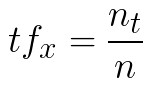
where x is the keyword, nt is the number of times x appears in the document and n is the total number of words in the document. 

The other metric Inverse Document Frequency or IDF measures how important is the keyword in the complete corpus of word. It is calculated with this formula

where x is the keyword, N is the total number of documents and dfx is the number of documents with keyword x in it.

Finally, we calculate the TF-IDF coefficient by multiplying these values. Keywords with high TF-IDF words are rare and significant. The cool thing is that sci-kit learn provides this function out of the box. Ok, but why do we need this? Well, we will use it to the representation of every movie in terms of its description, meaning in terms of its genre.

Loading and Preparing Data

Ok, now we know all the algorithms that we use, we can load data and pre-process it. We do so with DataHandler class:

It is a big class, but quite simple. Most of the logic happens in the constructor of the class. First, we load data from all CSV files in data_location. This is done in the _load_data method. Then genome tags and genome tag scores are merged and only tags with a score above the defined threshold are used. We use the threshold 0.3 as a default. After that, features are encoded, meaning every movie is connected with its tags, which are converted into a united string. This way we can apply TF-IDF to tags. In the end, we create the dataset by merging the average rating per movie with tags. This class has four public methods:

• get_tags_for_movie – returns tags for movie.
• get_average_rating_for_movie – returns average rating for a movie.
• get_movie_info – returns information about the movie based on the movie IDF.
• get_movie_info_with_title – returns information about the movies based on the movie title.

Here is how this class can be used. For example, I really like movie Snatch, so I want to find information about it in the dataset:

As an output I get a list of all movies that have word snatch in their title:

I can see that the movie I am looking for has ID 4011, so I call this function to get information about this movie:

TF-IDF Implementation

For the TF-IDF we use class TFIDF. Here it is:

All important things are done in the constructor. We use tf_idf from sci-kit learn to get extend dataset with descriptions based on tags. Also, we calculate the cosine similarity between each movie. Matrix movie_similarities contains information about how each movie relates to other movie based on the tags. This class provides one method find_top_5_simmilar_movies. This method returns 5 similar movies based on the movie Id. Here is how I can use this class to get movies that are similar to Snatch:

As the output we get:

Wow, that is really cool. Those movies are really similar to Snatch.

User Profiling

Finally, we need to profile each used, get her affinities and suggest similar movies based on that. We do that using UserProfiler class:

This class puts all together. It provides two methods get_user_ratings and get_user_recommendations. Here is how to use it to create recommendations for a user with ID 111:

Finally here is the output:

Conclusion

In this article, we explored how Content-Based Filtering works. For some recommendation systems, you will not need more than this technique, while for the others this is a perfect place to start and gather more data about the users. The main advantage is that only has to analyze the items and a single user’s profile, which makes it fairly simple to implement and it is not demanding when it comes to processing power. If we don’t have many users in the system, it will give pretty good results. Apart from that, it eliminates cold start problems. However, these systems can be imprecise exactly because it is not taking into consideration the behavior of other users in the system. For the same reason, it can over-specialize which leads to less diverse and novel recommendations.

Thank you for reading!