The code that accompanies this article can be found here.
In a previous couple of articles, we started exploring some of the basic machine learning algorithms. We covered some simple regression and classification algorithms. We also used other technologies like TensorFlow, Pytorch and SciKit Learn for the implementation and application of these algorithms and we used optimization techniques such as Gradient Descent. In this article, we focus on one very powerful algorithm – Support Vector Machine or SVM. SVM is one of the most popular machine learning algorithms and for a good reason. This algorithm proved over and over again to be really good for both – classification and regression and every machine learning engineer should have it in their toolbox. It is also applicable to linear and non-linear data. Before we dive into details and implementation of this algorithm let’s see datasets and libraries that we use in this article.
Are you afraid that AI might take your job? Make sure you are the one who is building it.
STAY RELEVANT IN THE RISING AI INDUSTRY! 🖖
Dataset and Prerequisites
Data that we use in this article is from PalmerPenguins Dataset. This dataset has been recently introduced as an alternative to the famous Iris dataset. It is created by Dr. Kristen Gorman and the Palmer Station, Antarctica LTER. You can obtain this dataset here, or via Kaggle. This dataset is essentially composed of two datasets, each containing data of 344 penguins. Just like in Iris dataset there are 3 different species of penguins coming from 3 islands in the Palmer Archipelago. Also, these datasets contain culmen dimensions for each species. The culmen is the upper ridge of a bird’s bill. In the simplified penguin’s data, culmen length and depth are renamed as variables culmen_length_mm and culmen_depth_mm.

Data that we use for the regression examples we use the famous Boston Housing Dataset. This dataset is composed 14 features and contains information collected by the U.S Census Service concerning housing in the area of Boston Mass. It is a small dataset with only 506 samples.
For the purpose of this article, make sure that you have installed the following Python libraries:
- NumPy – Follow this guide if you need help with installation.
- SciKit Learn – Follow this guide if you need help with installation.
Once installed make sure that you have imported all the necessary modules that are used in this tutorial.
import pandas as pd
import numpy as np
import matplotlib.pyplot as plt

from sklearn.model_selection import train_test_split
from sklearn.metrics import accuracy_score
from sklearn.preprocessing import StandardScaler
from sklearn.svm import LinearSVC, SVC, LinearSVR, SVR
Apart from that, it would be good to be at least familiar with the basics of linear algebra, calculus and probability.
SVM for Classification
Let’s first explore how this algorithm works for simple binary classification in order to understand how it functions. This means that we will consider only two classes form the PalmerPenguins dataset. As other machine learning algorithms SVM observers every feature vector as a point in a high-dimensional space. In its core, SVM puts all feature vectors on an imaginary n-dimensional plot and draws an imaginary n-dimensional line (a hyperplane) that separates examples with positive labels from examples with negative labels in the case of classification, or collects as much as samples as possible in case of regression. The hyperplane is defined by the function:

where x is the feature vector, w is feature weights vector with size same as x, and b is bias term. This is formula should be familiar from our journey through the Linear Regression or Logistic Regression. In the case of binary classification, which we consider at the moment, SVM requires that the positive label has a numeric value of 1, and the negative label has a value of -1. This means that predicted label for some feature vector x can be calculated using formula:

The function sign returns value 1 if the input is a positive number and -1 if the input is a negative value. So, SVM model, which during the training process should optimize w and b, can be described with the formula:

We can break this down and write it as:

This all looks very similar to the Logistic Regression approach. To better understand why this algorithm and what is the difference from Logistic Regression, let’s consider constraints under which algorithm operates:

On a graph that looks like this:

This means that SVM doesn’t only create a hyperplane, but it also constructs additional vectors which are defining margin. These vectors are called support vectors and the distance between the closest examples of two classes is called the margin. Hyperplane with support vectors is often referred to as street. This means that SVM tries to fit the best street between the samples of different classes. Unlike the Logistic regression which tries to fit the hyperplane as close as possible to these points, SVM tries to fit the hyperplane that is as far as possible form the samples but still separates classes successfully.
Note that a large margin leads to a better generalization, meaning the model will better classify new samples. However, notice that the margin is decided by the Euclidean norm of w (denoted by ||w|| in the image). This effectively means the smaller the weight vector w, the larger the margin and thus better generalization. To sum it up, training the SVM algorithm for classification means finding the value of w and b that makes margin as wide as possible while avoiding misclassification. Meaning, objective is defined as a constrained optimization problem:

where t(i) is –1 for negative samples and t(i) = 1 for positive samples. To be more precise, this optimization problem is a convex quadratic optimization problem with linear constraints. Such problems are known as Quadratic Programming (QP) problems. The solution for this type of problem is outside of the scope of this article. More information in Convex Optimization you can find here and more information for constraint optimization, in general, can be found here.
Preparing Data
As we mentioned for the classification examples we use PalmerPenguins dataset. However, since we want to do binary classification we need to do some preparations. First, we load the dataset, remove features that we don’t use in this article and remove the one class because we perform binary classification:
data = pd.read_csv('./data/penguins_size.csv')
data.head()
We remove all samples that are labeled with class ‘Chinstrap‘ and features that we don’t want to use (we use only culmen_length_mm and culmen_depth_mm).
data = data.dropna()
data = data.drop(['sex', 'island', 'flipper_length_mm', 'body_mass_g'], axis=1)
data = data[data['species'] != 'Chinstrap']
Then we separate input data and scale it:
X = data.drop(['species'], axis=1)
X = X.values
ss = StandardScaler()
X = ss.fit_transform(X)
After that, we extract output values and mark them with values -1 and 1, since the SVM algorithm requires that.
y = data['species']
spicies = {'Adelie': -1, 'Gentoo': 1}
y = [spicies[item] for item in y]
y = np.array(y)
Another thing that we remove is the 182nd sample form the dataset. Why? Well, this sample was in between classes and it kinda messed with points that we try to make, so we remove it and split data into training and test datasets:
# Remove sample that is too close
X = np.delete(X, 182, axis=0)
y = np.delete(y, 182, axis=0)

X_train, X_test, y_train, y_test = train_test_split(X, y, test_size=0.2, random_state=33)
That is it, our dataset is ready and here is what it looks when we plot it:
plt.figure(figsize=(11, 5))
plt.scatter(X[y == 0][:, 0], X[y == 0][:, 1], color='orange', label='Adelie')
plt.scatter(X[y == 1][:, 0], X[y == 1][:, 1], color='gray', label='Gentoo')
plt.legend();
Python Implementation
There are many methods to find the optimal w and b for the SVM. One of the most popular ones is Sequential Minimal Optimization (SMO) which is used by the SciKit Learn as well. In its core, the SMO algorithm splits the quadratic programming optimization problem into smaller ones. However, this algorithm is rather complicated so in this article, we implement a simpler one – The Pegasos algorithm. This algorithm uses stochastic gradient descent and it is defined like this:

So let’s implement this algorithm within the MySVM class:
class MySVM():
    def __init__(self, number_of_features, learning_rate=0.001):
        self.w = np.zeros(number_of_features + 1)
        self.learning_rate = learning_rate
        pass

    def __extend_input(self, X):
        ones = np.ones((X.shape[0], 1))
        return np.concatenate((ones, X), axis=1)

    def fit(self, X_train, y_train, epochs):
        X_train = self.__extend_input(X_train)

        for epoch in range(1, epochs):
            eta = 1/(self.learning_rate * epoch)
            fac = (1 - (eta * self.learning_rate)) * self.w

            for i in range(1, X_train.shape[0]):
                prediction = np.dot(X_train[i], self.w)

                if (y_train[i] * prediction) < 1 :
                    self.w = fac + eta * y_train[i] * X_train[i]
                else:
                    self.w = fac


    def predict(self, X_test):
        X_test = self.__extend_input(X_test)
        predictions = []

        for x in X_test:
            prediction = np.dot(self.w, x)
            prediction = 1 if (prediction > 0) else -1
            predictions.append(prediction)
        return np.array(predictions)
The implementation is fairly simple. In the constructor, we receive two parameters, number of features and learning rate. We need the number of features in order to initialize w. Note that we add 1 to that size because b is incorporated within w. That is why we need a private __extend_input method. This method is used to extend any input matrix with the column of ones. That is how b is implicitly modeled within the solution. Apart from that this class contains two public methods fit and predict following the blueprint dictated by big libraries like SciKit Learn.

The fit method handles the training process. In it, we first extend the training set and loop for a defined number of epochs. There we perform necessary calculations defined by the Pegasos algorithm. Finally, we update w for each sample in the training set. The predict method just extends the test set and multiplies it with w. If the result is larger than 0 it appends label 1, otherwise, it appends label -1. As you may notice, unlike Logistic Regression, SVM doesn’t output probabilities for each class. It is easy to use this class:
model = MySVM(X_train.shape[1])
model.fit(X_train, y_train, 10000)

preditions = model.predict(X_test)
print(accuracy_score(preditions, y_test))1.0In the end, we get that accuracy of 100%.
Using SciKit Learn
Of course, we can use SciKit Learn implementation of this classifier. Since our data is linearly separable we can use LinearSVC class:
lsvc_model = LinearSVC(C=1, loss="hinge")

lsvc_model.fit(X_train, y_train)

lsvc_preditions = lsvc_model.predict(X_test)
print(accuracy_score(lsvc_preditions, y_test))1.0Hyperparameter C is used to control the wideness of the street. Smaller C value leads to a wider street, however, it leads to more margin violations. This means that samples could end up that end up in the middle of the street or even on the wrong side. For loss function, we used hinge loss. This loss is effective for SVM algorithms. It is defined with the formula: max(0, 1 – t). Its derivative is –1 if t < 1 and 0 if t > 1.
Alternatively, we can use the SVC class:
svc_model = SVC(kernel="linear", C=1)

svc_model.fit(X_train, y_train)

svc_preditions = svc_model.predict(X_test)
print(accuracy_score(svc_preditions, y_test))1.0We got the same result, ie. 100% accuracy, but you may notice kernel hyperparameter, which is going to be explained in the next chapter. Anyhow, here are the compared results of all three algorithms within pandas data frame:
pd.DataFrame({
    'Actual Value': y_test,
    'My SVM Predictions': preditions,
    'LinearSCV Predictions': lsvc_preditions,
    'SVC Predictions': svc_preditions,
})
If we plot it out these models, here is what we get:

Notice the difference between a linear function that separates two classes between our and SciKit Learn implementation. This is caused by different algorithms that implementations used.
Non-Linear Data
Thus far we observed a pretty nice example, data that is linearly separable. In reality, this is almost never the case. So, let’s consider other classes from the PalmerPenguins dataset and load Adelie and Chinstrap classes.
data = pd.read_csv('./data/penguins_size.csv')
data = data.dropna()
data = data.drop(['sex', 'island', 'flipper_length_mm', 'body_mass_g'], axis=1)
data = data[data['species'] != 'Gentoo']

X = data.drop(['species'], axis=1)

ss = StandardScaler()
X = ss.fit_transform(X)

y = data['species']
spicies = {'Adelie': -1, 'Chinstrap': 1}
y = [spicies[item] for item in y]
y = np.array(y)

X_train, X_test, y_train, y_test = train_test_split(X, y, test_size=0.2, random_state=33)

plt.figure(figsize=(11, 5))
plt.scatter(X[y == -1][:, 0], X[y == -1][:, 1], color='orange', label='Adelie')
plt.scatter(X[y == 1][:, 0], X[y == 1][:, 1], color='gray', label='Gentoo')

plt.legend();
This time it is not so easy to separate classes with just a straight line. Data is a bit scrambled, so what should we do in these situations when data is not linear? Here we can apply probably the greatest SVM advantage – kernel trick. This technique gives you the possibility to get the same result as if you were using polynomial features without actually having to add them. Kernels are just functions that map low-dimensional non-linearly-separable data into a linearly-separable high-dimensional data. Meaning, in our case, we map our 2D data which is not linearly separable into 3D data that is.

However, we don’t know which mapping works for our data the best, so if we would map all the vectors into a higher dimension and then apply SVM to it that would be very inefficient. That is where the kernel trick comes into play. In essence, it uses kernels to work in higher-dimensional spaces without doing this transformation explicitly. So, let’s use different kernels on our dataset. First, we use the polynomial kernel and here is the result that we get.
svc_model_poly = SVC(kernel="poly", C=0.6)

svc_model_poly.fit(X_train, y_train)

svc_poly_preditions = svc_model_poly.predict(X_test)
print(accuracy_score(svc_poly_preditions, y_test))0.9069767441860465As you can see accuracy is around 90%. That is not bad, but can it get better. One of the most popular kernel functions is Gaussian RBF kernel defined by the formula:

It is a bell-shaped function varying from 0 to 1 and it is often used for adding features using similarity features method. Notice the parameter gamma. It is defining how wide the bell-curve is and this essentially the hyperparameter of the SVM. In essence, when we use this kernel we create a gaussian bell-curve in 3-dimensional space, in this example (since our data is in 2-dimensional space), around the chosen landmark.
Then all points are mapped from 2-dimensional space to 3-dimensional space, but every point is mapped to this curve. That is how we ensure that data is linearly separable in 3-dimensional space. Then SVM is applied. Of course kernel trick is applied so we don’t have to do all of these calculations, so the algorithm is pretty efficient. Let’s use RBF:
svc_model_rbf = SVC(kernel="rbf", gamma=.5, C=0.1)

svc_model_rbf.fit(X_train, y_train)

svc_rbf_preditions = svc_model_rbf.predict(X_test)
print(accuracy_score(svc_rbf_preditions, y_test))0.9767441860465116The accuracy is around 97%. That is much better than the polynomial kernel. If we visualize both approaches, we get something like this:

You can imagine 3D Gaussian bell-curve coming out of your screen in the RBF example if you will 🙂
SVM for regression – SVR
SVM for regression is not so different from the one for the classification. In essence, all the practices that we learned for classification stand for the regression as well, with one major difference. For the classification SVM tried to fit the largest street among the samples of different classes, without violating margins. In regression, SVM tries to fit as many samples as possible on the street, while minimizing number of the samples of the street. The wideness of the street is controlled by hyperparameter – epsilon.
Preparing Data
For regression example, we use the Boston housing dataset. This dataset contains 14 features, of which we use 2. Our goal in this example is to predict the value of the property based on the age of the occupant. So, we remove all other features:
data = pd.read_csv('./data/boston_housing.csv')
data.head()

data = data.dropna()

X = data['lstat'].values
X = X.reshape(-1, 1)

y = data['medv'].values

X_train, X_test, y_train, y_test = train_test_split(X, y, test_size=0.2, random_state=33)
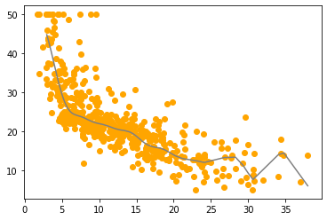
Here is how that looks like when we plot it:

As you can see this is the case of non-linear regression. So, let’s try to create a model that will best fit this data.
Using SciKit Learn
We know that regression in this example is non-linear, but for educational purposes, we start with linear SVM regression.
lsvr_model = LinearSVR(epsilon=1.5, max_iter=10000)
lsvr_model.fit(X_train, y_train)

lsvr_predictions = lsvr_model.predict(X_test)

pd.DataFrame({
    'Actual Value': y_test,
    'LinearSVR Prediction': lsvr_predictions,
})
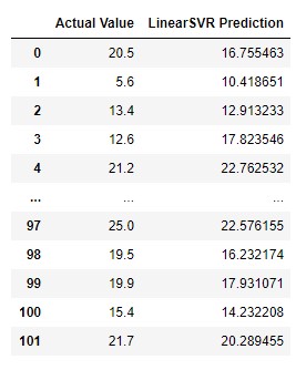
The results are, well, mixed. Sometimes they are not that bad, but sometimes they are far off. It looks like a random guess. When we plot it out, the model makes more sense:

It is interesting. We can almost see how SVM works and how it tried to fit as many points around that line. Of course, we can improve the results by using other kernels. Here is how we use polynomial kernel:
psvr_model = SVR(kernel="poly", degree=2, C=100, epsilon=0.1)
psvr_model.fit(X_train, y_train)

psvr_predictions = psvr_model.predict(X_test)

pd.DataFrame({
    'Actual Value': y_test,
    'LinearSVR Prediction': lsvr_predictions,
    'PolySVR Prediction': psvr_predictions
})
Compared to linear model results are somewhat better. When we plot the model, here is what we get:

Notice the degree parameter in the constructor of the SVR class. Try changing its value of this parameter and the value of epsilon to get better results. Finally, let’s use the RBF kernel:
svr_rbf_model = SVR(C=100, gamma=0.1, epsilon=.1)
svr_rbf_model.fit(X_train, y_train)

svr_rbf_predictions = svr_rbf_model.predict(X_test)

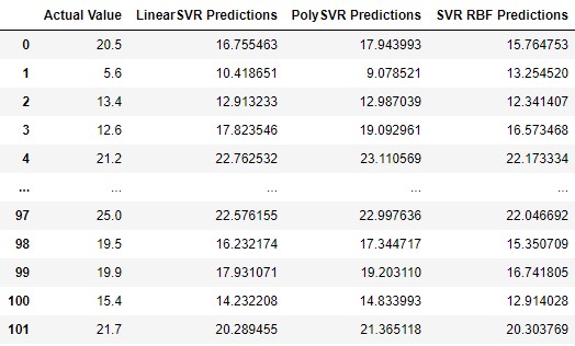
pd.DataFrame({
    'Actual Value': y_test,
    'LinearSVR Predictions': lsvr_predictions,
    'PolySVR Predictions': psvr_predictions,
    'SVR RBF Predictions': svr_rbf_predictions
})
This model gets the best results. Let’s plot it:

Conclusion
In this article, we covered large topic of SVM. We had a chance to see how it works for classification and for regression. We also saw how we can handle linear data and how we can handle non-linear data using kernel trick. SVM is one amazing algorithm which is important part of your Machine Learning toolbox.
Thank you for reading!

Nikola M. Zivkovic
CAIO at Rubik's Code
Nikola M. Zivkovic a CAIO at Rubik’s Code and the author of book “Deep Learning for Programmers“. He is loves knowledge sharing, and he is experienced speaker. You can find him speaking at meetups, conferences and as a guest lecturer at the University of Novi Sad.
Rubik’s Code is a boutique data science and software service company with more than 10 years of experience in Machine Learning, Artificial Intelligence & Software development. Check out the services we provide.


Trackbacks/Pingbacks