Python for Data Science - NumPy & Pandas Cheatsheet

We always get a lot of questions about where one should start when getting into the field of machine learning and data science. Always, our answer is that mathematics and the basics of Python are mandatory. In fact, you can subscribe to our blog and get free Math for Machine Learning guide here. However, we haven’t covered Python basics on this blog, so we decided to change that. In this article, we learn about two libraries without Data Scientists would be lost – NumPy and Pandas. You can kickstart your data science career with this two-part cheatsheet.

Here is what this tutorial is covering:

NumPy
Pandas

1. NumPy

This library is the granddad of all other important data science libraries. It is a fundamental library for scientific computing in Python. Basically, all other libraries like Pandas, Matplotlib, SciKit Learn, TensorFlow, Pytorch are built on top of it. In its essence, it is a multidimensional array library. So simple? As you probably already know, linear algebra is one of the main building blocks of machine learning. It makes it all possible. Manipulating vectors (represented as arrays in Python) and matrixes is much easier with NumPy.

Ok, but why use it over Python standard lists? Among several reasons the main one is speed. Unlike lists, NumPy uses fixed types and that is where the speed comes from. For example, if we observe a simple 32 bits integer, Python lists would store much more information than NumPy. Built-in integer type stores the following information: size, reference count, object type, object value. So instead of just 4 bytes that NumPy would use, the list use ~28 bytes.

Apart from that Numpy uses contiguous memory in heap, unlike lists. This also brings effective cache utilization. In a nutshell, one of the reasons that NumPy is faster than lists is that it uses less memory and fixed types. Another benefit NumPyhas way more operations and features than lists. NumPy comes with Anaconda Python distribution, so if you installed Anaconda you are good to go. Otherwise Install it with command:

pip install numpy

To import NumPy in your project, just use:

import numpy as np

1.1 NumPy Array

NumPy array is the main building block of the NumPy. In data science, it is often used to model and abstract vectors and matrixes. Here is how you can initialize simple array:

array = np.array([1, 2, 3])
print(array)

[1 2 3]

Matrix (2d array) can be initialized like this:

twod_array = np.array([[1, 2, 3], [4, 5, 6]])
print(twod_array)

[[1 2 3]
[4 5 6]]

You can get a lot of information about NumPy Array. For example, if you need dimensions of it you can call the ndim attribute:

print(array.ndim)
print(twod_array.ndim)

1
2

However, more often you will need the shape of the array, meaning when you are working on machine learning and deep learning applications shapes of the matrixes give you information about the input and output of your architecture. You can get a shape like this:

print(array.shape)
print(twod_array.shape)

(3,)
(2, 3)

As you can see from here, the array is a one-dimensional array with three elements, while twod_array is a 2×3 matrix. Apart from that, you can always get the type of the array by checking the dtype attribute. This attribute can be used during initialization of the array as well to define the type of array:

array = np.array([1, 2, 3], dtype='int16')
array.dtype

dtype('int16')

You may be interested in how many elements there are in some array, and what is its memory footprint. Here is how you can do that with the attributes itemsize, size and nbytes:

print(f"**********************************************************************")
print(f"Array has type {array.dtype} which means that every item takes {array.itemsize} bytes.")
print(f"2D Array has {array.size} elements.")
print(f"Array total size is {array.nbytes} bytes.")
print(f"**********************************************************************")
print(f"2D Array has type {twod_array.dtype} which means that every item takes \
	{twod_array.itemsize} bytes.")
print(f"2D Array has {twod_array.size} elements.")
print(f"2D Array total size is {twod_array.nbytes} bytes.")

**********************************************************************
Array has type int16 which means that every item takes 2 bytes.
2D Array has 3 elements.
Array total size is 6 bytes.
**********************************************************************
2D Array has type int32 which means that every item takes 4 bytes.
2D Array has 6 elements.
2D Array total size is 24 bytes.

1.2 Reading and Updating Elements, Rows and Columns with Indexes

There are many options when it comes to manipulation with the arrays in the NumPy. Let’s initialize a matrix that we use for these experiments:

x = np.array([[1, 2, 3, 4, 5, 6, 7],[8, 9, 10, 11, 12, 13, 14]])
print(x)
print(f"Shape:{x.shape}")

[[ 1  2  3  4  5  6  7]
[ 8  9 10 11 12 13 14]]
Shape:(2, 7)

Sometimes you need a specific element from the array. That is done with indexes. For example, you want to get the fourth element from the second row from the array x. That is done like this:

print("The fourth element of the second row is:")
print(x[1, 3]) # Indexes are starting from 0

The fourth element of the second row is:
11

The first number in the [] brackets is the index along the first dimension of the array, while the second number is the index along the second dimension of the array x. Note that the indexes in Python are starting from 0. Let’s practice it and get the sixth element from the first row:

print("The sixth element of the first row is:")
print(x[0, 5]) # Indexes are starting from 0

The sixth element of the first row is:
6

Another way to access the same element is by using negative indexes. These indexes indicate that we “count” from the back of the array. It is one neat trick:

print("The sixth element of the first row is:")
print(x[0, -2]) # Negative indexes go from the back of the array

The sixth element of the first row is:
6

If we want to get a complete row as a separate NumPy array, we can do it like this:

print("The first row is:")
print(x[0, :])

The first row is:
[1 2 3 4 5 6 7]

The ‘:’ indicate that everything should be taken from that dimension, ie. axis. We can utilize negative indexes too:

print("The second row is:")
print(x[-1, :]) # Negative indexes go from the back

The second row is:
[ 8  9 10 11 12 13 14]

In the same way, by using ‘:’, we can get complete columns as a separate NumPy array:

print("The first column is:")
print(x[:, 0])

The first column is:
[1 8]

The cool thing is that we can get subset of this matrix. For example, if we want the first three elements from the first row, we can do so like this:

print("The first 3 elements from the first row:")
print(x[0, 0:3])

The first 3 elements from the first row:
[1 2 3]

Indexing can be used for updating values in the array too:

# Replace the value of the 6th element in the second row with 33
x[1, 5] = 33
print(x)

[[ 1  2  3  4  5  6  7]
[ 8  9 10 11 12 33 14]]

In the same way, you can do a bulk update:

# Bulk Update 
# Replace elements from third to fifth in the first row with value 56

x[0, 2:5] = 56
print(x)

[[ 1  2 56 56 56  6  7]
[ 8  9 10 11 12 33 14]]

Finally, another cool thing with the NumPy array is Boolean indexing. This means that you can get a true/false value for each element in the array based on some condition. For example, let’s check out wich elements in array x are larger than 10:

x > 10

array([[False, False,  True,  True,  True, False, False],
       [False, False, False,  True,  True,  True,  True]])

1.3 NumPy Array Initialization

NumPy provides numerous functions for array initialization. For example, if you need a matrix with all zeros, you can do so like this:

# All zeros 5x6 matrix 
zeros = np.zeros((5, 6))
print(zeros)

[[0. 0. 0. 0. 0. 0.]
 [0. 0. 0. 0. 0. 0.]
 [0. 0. 0. 0. 0. 0.]
 [0. 0. 0. 0. 0. 0.]
[0. 0. 0. 0. 0. 0.]]

Or, if you need a matrix with all ones:

# All ones 5x6 matrix 
ones = np.ones((5, 6))
print(ones)

[[1. 1. 1. 1. 1. 1.]
 [1. 1. 1. 1. 1. 1.]
 [1. 1. 1. 1. 1. 1.]
 [1. 1. 1. 1. 1. 1.]
 [1. 1. 1. 1. 1. 1.]]

Sure, you can initialize a complete matrix with a certain number:

# Any other number 5x6 matrix 
ninenine = np.full((5,6), 99)
print(ninenine)

[[99 99 99 99 99 99]
 [99 99 99 99 99 99]
 [99 99 99 99 99 99]
 [99 99 99 99 99 99]
 [99 99 99 99 99 99]]

The interesting thing about the full method is that there is a variation called full_like. This function picks up dimensions from another array that is already created and creates a new matrix with a defined value. Check it out:

# Any other number with dimensions from another array (full_like)
fivefive = np.full_like(x, 55)
print(fivefive)

[[55 55 55 55 55 55 55]
[55 55 55 55 55 55 55]]

If you need a matrix with random values, NumPy gets you covered. There is a whole submodule called random, using which you can create different random values:

# 5x6 matrix with random float numbers
randomize = np.random.rand(5, 6)
print(randomize)

[[0.96285976 0.00931921 0.61453111 0.6846065  0.17965427 0.92548501]
 [0.78119724 0.25421679 0.33713402 0.78393532 0.44122679 0.24001506]
 [0.27472269 0.99649043 0.48591665 0.13464157 0.39398014 0.16291523]
 [0.48315635 0.33255073 0.16103341 0.55914281 0.59750496 0.80263915]
 [0.08985945 0.84173854 0.87351364 0.3576588  0.3742723  0.00807349]]

You can do the same thing with integers:

# 5x6 matrix with random int numbers
randomizeint = np.random.randint(6, size=(5,6))
print(randomizeint)

[[5 0 1 3 5 4]
 [3 5 3 4 1 5]
 [1 3 1 0 3 4]
 [1 3 2 3 0 4]
 [2 1 2 4 3 2]]

To create identity matrix, you can use identity function, which receives dimensions of identitiy matrix:

# 3x3 identity matrix
identity = np.identity(3)
print(identity)

[[1. 0. 0.]
 [0. 1. 0.]
 [0. 0. 1.]]

Also, there are multiple ways to create new matrixes from arrays. This can be done with methods like repeat and stack:

# Repeat
print(f"*************************Initial*********************************")
initial = np.array([[2, 11, 9]])
print(initial)

print(f"*************************Expended1*******************************")
expanded1 = np.repeat(initial, 3, axis=1)
print(expanded1)

print(f"*************************Expended2*******************************")
expanded2 = np.repeat(initial, 3, axis=0)
print(expanded2)

*************************Initial*********************************
[[ 2 11  9]]
*************************Expended1*******************************
[[ 2  2  2 11 11 11  9  9  9]]
*************************Expended2*******************************
[[ 2 11  9]
 [ 2 11  9]
 [ 2 11  9]]

As you can see repeat has an axis parameter, using which you can define by which axis array is going to be repeated. The stack method is similar, but it is more useful, since with it you can merge multiple arrays:

# Stack
array1 = np.array([1, 2, 3])
array2 = np.array([4, 5, 6])

stacked = np.vstack([array1, array2])
print(stacked)

[[1 2 3]
[4 5 6]]

Finally, arrays can be reshaped using the reshape method. This functionality is very useful for deep learning applications:

# Reshape
stacked.reshape((3, 2))

array([[1, 2],
       [3, 4],
       [5, 6]])

1.4 Operations with Scalars

With NumPy Arrays it is quite easy to perform simple operations like addition, multiplication and division with the scalars (ie. simple numbers). Let’s observe NumPy array y:

y = np.array([1, 2, 3, 4, 5, 6])
print(y)

[1 2 3 4 5 6]

Or if we want to subtract number 3 from each element:

print(y - 3)

[-2 -1  0  1  2  3]

Multiplication? You name it:

print(y * 3)

[ 3  6  9 12 15 18]

The division is supported too:

print(y / 3)

[0.33333333 0.66666667 1.         1.33333333 1.66666667 2.        ]

You can do exponential operations as well:

print(y ** 3)

[  1   8  27  64 125 216]

1.5 Linear Algebra with NumPy

As we mentioned, NumPy is quite a useful library for linear algebra. This means that we can easily do operations with other arrays. Let’s say that we want to add some array to the array y:

z = np.array([6, 5, 4, 3, 2, 1])
print(y + z)

[7 7 7 7 7 7]

Or subtract values of one array from another array:

print(y - z)

[-5 -3 -1  1  3  5]

You can do element-wise multiplication of two arrays:

print(y * z)

[ 6 10 12 12 10  6]

Or divide one array with another:

print(y / z)

[0.16666667 0.4        0.75       1.33333333 2.5        6.        ]

If you want to multiply two matrixes, this can be done with matmul method:

x = np.ones((2, 3))
y = np.full((3, 2), 6)

print(x)
print(y)

[[1. 1. 1.]
 [1. 1. 1.]]
[[6 6]
 [6 6]
 [6 6]]

# Matrix multiplication
np.matmul(x, y)

array([[18., 18.],
       [18., 18.]])

If you need determinant of some matrix, that can be done too:

# Derminant of 3x3 identity matrix
np.linalg.det(np.identity(3))

1.0

1.6 Basic Statistics with NumPy

There are many statistics options that you can perform with NumPy. In this tutorial, we cover only the basics. Let’s create an array from random integer values:

x = np.random.randint(10, size=11)
print(x)

[9 5 5 3 0 2 8 5 2 2 2]

For this array (or any other for that matter) we can quickly get max value:

np.max(x)

Or minimal value:

np.min(x)

Also, we can get the mean and median value of the array wich is quite usefull:

np.mean(x)

1.0

np.median(x)

1.0

1.6 Trigonometry with NumPy

Finally, Numpy has some really useful options when it comes to Trigonometry, like getting sine and cosine of values in the array:

np.sin(y)

array([[-0.2794155, -0.2794155],
     [-0.2794155, -0.2794155],
     [-0.2794155, -0.2794155]])

np.cos(y)

array([[0.96017029, 0.96017029],
     [0.96017029, 0.96017029],
     [0.96017029, 0.96017029]])

2. Pandas

Pandas is one of the popular libraries that is built on top of NumPy. Some people are considering the most important tool of the data analysts and indeed it is quite useful. There are many things you can do with this library, including data pre-processing and data cleanup. It is one of the best tools for exploratory data analysis and feature engineering. Pandas’ data structures are fast, flexible and designed to make data analysis easy.

It is part of Anaconda Python Distribution, but you can install it with pip too.

Let’s see what it is all about!

2.1 Pandas Series

Series are the basic building block of Pandas library. They can be observed as NumPy array, but with indexes that can be labeled. For example, you can create a simple series like this:

x = pd.Series(np.random.rand(3), index= ['a', 'b', 'c'])
x

a    0.661511
b    0.441051
c    0.139237
dtype: float64

We may loosely define it as a “label indexed array”. The indexing work the same way as with NumPy arrays, with the exception that you can use labels as indexes:

print(x[0])

0.6615108128588524

print(x['a'])

0.6615108128588524

In the same way that we sliced the NumPy Array with ‘:’, the same thing can be done here:

print(x[:2])

a    0.661511
b    0.441051
dtype: float64

2.2 Pandas DataFrames

If the Series are arrays DataFrames are matrices. DataFrames have rows and columns, and each of them is labeled. Here is how we create one:

df = pd.DataFrame(x, columns = ['Column 1'])
df

There is various information that DataFrame provides out of the box, like shape:

df.shape

(3, 1)

At any moment we can get index information:

df.index

Index(['a', 'b', 'c'], dtype='object')

The same goes for the Columns info:

df.columns

Index(['Column 1'], dtype='object')

As well as the number of instances per column:

df.count()

Column 1    3
dtype: int64

Finall, complete description of the DataFrame can be retrieved like this:

df.info()

<class 'pandas.core.frame.DataFrame'>
Index: 3 entries, a to c
Data columns (total 1 columns):
 #   Column    Non-Null Count  Dtype  
---  ------    --------------  -----  
 0   Column 1  3 non-null      float64
dtypes: float64(1)
memory usage: 128.0+ bytes

If you need to extend your DataFrame with another column that can be done fairly easy:

df['Column 2'] = df['Column 1'] * 3
df

2.3 Reading Operations

The cool thing about Pandas is that there are multiple options for selecting columns, rows as well as specific elements. For example, if we want to select one element, there are multiple ways we can do that. We can use labels:

df.loc['a', 'Column 1'] # This funcion is label based

0.6615108128588524

There is also function iat, which we can use if we know the position of the element in the DataFrame:

df.iat[0, 0] # Use iat if you only need to get or set a single value

0.6615108128588524

With labels, we can select the whole column. This operation returns Series object:

df['Column 1'] # Returns a Series by columb label

a    0.661511
b    0.441051
c    0.139237
Name: Column 1, dtype: float64

Rows can be selected with iloc method:

df.iloc[0] # Select Row

Column 1    0.661511
Column 2    1.984532
Name: a, dtype: float64

Boolean indexing is available in Pandas too, but there is more control since you can use each column separately:

df['Column 1'] > 0.5 # Boolean Indexing

a     True
b    False
c    False
Name: Column 1, dtype: bool

2.4 Dropping rows/columns

The drop method is the method that we use when we want to remove the series from DataFrame. Series can be row or column. This is controlled by the axis parameter. Here is how we can remove row:

df1 = df.drop('c', axis=0) #Axis 0 indicates that this is a row
df1

The column can be removed if we use axis=1:

df1 = df1.drop('Column 2', axis=1) # Axis 1 indicates that this is a column
df1

2.5 Sorting and Ranking

Pandas is sometimes compared with Excel, because of the tabular operations you can do with it. Sorting and rankig are one of them. For example, you can sort data by index:

df.sort_index()

In our example DataFrame looks exactly the same, however, if our index labels were not sorted, this method would do the trick. The sorting can be done by each column:

df.sort_values(by='Column 2')

The another useful thing is adding ranks to the values which can be done with rank method:

df.rank()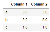

2.6 Basic Statistics with Pandas

Pandas provide several options for statistics of each column and row. The basic information about each column can be retrieved with the describe method:

df.describe()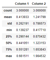

As you can see all the important points are here, like mean, median, standard deviation, max, min, Q1 and Q3. It is a pretty good indication of the distribution of each column. Almost, every point from the table above has a separate function that you can use in case you need it. If you need mean value of a column use mean function:

df.mean()

Column 1    0.413933
Column 2    1.241799
dtype: float64

For median value, there is median function:

df.median()

Column 1    0.441051
Column 2    1.323153
dtype: float64

Maximum and minimum have functions max and min respectively:

df.min()

Column 1    0.139237
Column 2    0.417710
dtype: float64

df.max()

Column 1    0.661511
Column 2    1.984532
dtype: float64

You can also get the index of the maximal and minimal value, using idxmax and idxmin respectevly:

df.idxmin()

Column 1    c
Column 2    c
dtype: object

df.idxmin()

Column 1    a
Column 2    a
dtype: object

Apart from that you can get the sum of each column using sum() method:

df.sum()

Column 1    1.241799
Column 2    3.725396
dtype: float64

Or get cumulative sum usig cumsum method:

df.cumsum()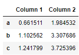

2.7 Using Functions with DataFrames

If you want to make some sort of transformations on the data in the DataFrame you can utilize functions. One way is to use unnamed lambda functions and apply the method:

df.apply(lambda x: x + 3)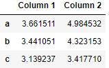

2.8 Manipulate Data from CSV

Tabular data is often stored in CSV files. We can load this tabular data in the DataFrames using the read_csv function. For example, let’s load data from PalmerPenguin dataset:

data = pd.read_csv('./data/penguins_size.csv')
data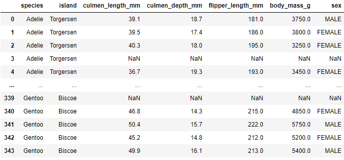

Then you can get more infromation and manipulate this data with Pandas:

data.describe()

Once you are done you can store data into some new csv file like this:

data.to_csv('./data/new_file.csv')

2.9 Manipulate Data from SQL

Tabular data often comes from the SQL database. In order to load this data into DataFrame, you can use SQL-Alchemy library in combination with Pandas:

from sqlalchemy import create_engine
engine = create_engine('sqlite:///:memory:')

pd.read_sql('SELECT * FROM palmer_penguins;', engine)
pd.read_sql_table('palmer_penguins', engine)
pd.read_sql_query('SELECT * FROM palmer_penguins;', engine)

As you can see you can send SQL queries for specific tables. Also you can write data to SQL like this:

data.to_sql('penguin_data', engine)

Conclusion

In this article, we covered the basics of two fundamental Data Science libraries – NumPy and Pandas. Of course, we were not able to go through all options that these libraries provide, but we find that these cheatsheets can be a valid guide for begginers and as a refference guide for more expirienced data scientist.

Thank you for reading!

Nikola M. Zivkovic

CAIO at Rubik's Code

Nikola M. Zivkovic a CAIO at Rubik’s Code and the author of book “Deep Learning for Programmers“. He is loves knowledge sharing, and he is experienced speaker. You can find him speaking at meetups, conferences and as a guest lecturer at the University of Novi Sad.

Rubik’s Code is a boutique data science and software service company with more than 10 years of experience in Machine Learning, Artificial Intelligence & Software development. Check out the services we provide.

Python for Data Science – NumPy & Pandas Cheatsheet