
From Netflix, Google, and Amazon, to smaller webshops, recommendation systems are everywhere. In fact, this type of system represents probably one of the most successful business applications of Machine Learning. Their ability to predict what users would like to read, watch and buy proved to be good not only for the business but for the users as well. For users, they provide a way to explore product space and for businesses they provide an increase in user engagement and more knowledge about the customers. Also, these systems are widespread and existing in almost every big cloud platform. When we think of YouTube video recommendations, they are there. Netflix menus with suggested series, they are turning the wheels behind the scene. Gmap suggested routes? You can bet. These systems became one of the building blocks of our industry and it would be bad not to know anything about them. In this article, we get familiar with these systems and see how we can build one using ML.NET.

Are you afraid that AI might take your job? Make sure you are the one who is building it.
STAY RELEVANT IN THE RISING AI INDUSTRY! 🖖
The topics covered in this article are:
1. Dataset and Prerequisites
Everyone loves Netflix. One reason for it is that their recommendations are top-notch. The company invested a lot in this. They are famous for their Netflix Prize competition, where engineers try to predict user ratings for films, based on previous ratings without any other information about the users or films. They even provided a dataset, a training data set of 100,480,507 ratings that 480,189 users gave to 17,770 movies. Each sample in the dataset is formatted as a set of four features: user ID, movie ID, Grade, Date of Grade. The user ID and movie ID features are integer IDs, while grades are from 1 to 5. In general, in this article, we will not use dates. Here is how that data looks like.

The implementations provided here are done in C#, and we use the latest .NET 5. So make sure that you have installed this SDK. If you are using Visual Studio this comes with version 16.8.3. Also, make sure that you have installed the following packages:
$ dotnet add package Microsoft.ML
$ dotnet add package Microsoft.ML.Recommender
You can do the same from the Package Manager Console:
Install-Package Microsoft.ML
Install-Package Microsoft.ML.Recommendation
Note that this will install default Microsoft.ML package as well. You can do a similar thing using Visual Studio’s Manage NuGetPackage option:

If you need to catch up with the basics of machine learning with ML.NET check out this article.
2. Types of Recommendation Systems
As we mentioned, the Netflix dataset contains information on how a user rated a movie. Based on this, how do we create a recommendation for that user? We need to consider some features of the movie that the user has watched and ranked, and then recommend similar items. Alternately, we could consider finding similar users based on those rankings and suggest items that those users purchased. But what does it mean that two items are similar? What does it mean that two users are similar? How to calculate that and present that similarity in some mathematical terms?

Different types of recommendation systems take different approaches to these questions. In general, there are four types of recommendation systems:
- Content-Based Recommendation Systems – This type of recommendation system is focused, well, on content. Meaning they use only features and information from the items and based on them create recommendations for the user. They don’t take into account information from other users.
- Collaborative Filtering Recommendation Systems – The biggest power of recommendation systems is that they can suggest items for users based on their behavior on a certain platform or based on the behavior of other users of the same platform. For example, Netflix suggests your next series to binge, based on the series you’ve previously watched, but based on the series that users that watched and liked the same content as you too.
- Knowledge-Based Recommendation Systems – This type of recommendation system use explicit knowledge about the user’s preferences, items, and or recommendation criteria. In this scenario, recommendation systems would ask a user about their preferences and based on that feedback build recommendations.
- Hybrid Solutions Recommendation Systems – Often, we use a combination of all types for some custom solutions.
If you want to learn more about how each of these systems works check out this article. From these three types, the first two are used most often and the most popular. In practice, it can happen that we build hybrid solutions to get better results.
ML.NET supports only collaborative filtering, or to be more specific – matrix factorization. That is why in this article we focus on this type of recommendation system. Let’s learn more about how these systems function under the hood.
3. Collaborative Filtering Intuition
One of the most popular techniques to create recommendation systems is Collaborative Filtering. Unlike Content-Based Filtering, this approach places users and items are within a common embedding space along dimensions (read – features) they have in common. For example, let’s consider two users from Netflix and shows that they rated.

We can present that like this in TensorFlow (no worries, we will not go into TensorFlow details, this is just for example purposes :)):
users_tv_shows = tf.constant([
                [10,  2,  0,  0, 0, 6],
                [0, 1,  0,  2, 10, 0]],dtype=tf.float32)
Now, we ca take the features of each show, which is just k-hot encoding of the genre:

Or in TensorFlow:
tv_shows_features = tf.constant([
                [0, 0, 1, 0, 1],
                [1, 0, 0, 0, 0],
                [1, 0, 0, 0, 0],
                [0, 1, 0, 1, 0],
                [0, 0, 1, 0, 0],
                [0, 1, 0, 0, 0]],dtype=tf.float32)
Then we can do simple dot product of these matrices and get the affinities of each user:
users_features = tf.matmul(users_tv_shows, tv_shows_features)
users_features = users_features/tf.reduce_sum(users_features, axis=1, keepdims=True)

top_users_features = tf.nn.top_k(users_features, num_feats)[1]
for i in range(num_users):
    feature_names = [features[int(index)] for index in top_users_features[i]]
    print('{}: {}'.format(users[i],feature_names))
User1: ['Comedy', 'Drama', 'Sci-Fi', 'Action', 'Cartoon']
User2: ['Comedy', 'Sci-Fi', 'Cartoon', 'Action', 'Drama']We can see that the top feature for both users is Comedy, which means they like similar stuff. What have we done here? Well, we not only described items in terms of the mentioned genres, but we have done the same for each user with the same terms. The meaning for a User1, for example, is that she likes Comedy 0.5 but he likes Action 0.1. Note that if we multiply users’ embedding matrix with the transpose item embedding matrix we will recreate the user-item interaction matrix. Now, this works well for simple examples with few users and items. However, as more items and users are added to the system it becomes unscalable. Also, how can we be so sure that the features that we picked are the relevant ones? What if there are some latent features, that we are unable to recognize. So how can we pick the correct features then? This brings us to the matrix factorization.
4. Matrix Factorization Intuition
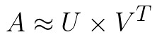
We mentioned that human-defined features for items and users might not be the best option overall. Fortunately, these embeddings can be learned from data. This means that we don’t manually assign features to the items and to the users, but we will use the user-item interaction matrix to learn the latent factors that best factorize it. As in the previous mind-exercise, this process results in a user factor embedding and item factor embedding matrixes. Technically, we are compressing a sparse user-item interaction matrix and extracting latent factors (something like PCA). That is what matrix factorization is all about, being able to factorize a matrix into two smaller matrixes using which we can reconstruct the original one:
Your content goes here. Edit or remove this text inline or in the module Content settings. You can also style every aspect of this content in the module Design settings and even apply custom CSS to this text in the module Advanced settings.

Similar to the other dimensionality reduction techniques, the number of latent features is a hyperparameter that we can change and use it for a tradeoff between more information compression and more reconstruction error. In order to make a prediction, we can do it in two ways. We can either take the dot product of a user with the item factors or the dot product of an item with the user factors. Matrix factorization helps us with one more problem. Imagine that you have thousands of users in our system and you want to calculate the similarity matrix between them. That matrix would get quite big. Matrix factorization compresses that information for us.
4.1 Matrix Factorization Algoritms
There are several good Matrix Factorization out there. So let’s explore some of the more popular ones. A couple of years back, Netflix published a $1M competition for recommendation systems. The goal was to improve the accuracy of their system based on users’ ratings. The winner used the SVD (Singular Value Decomposition) algorithm to get the best results. This algorithm is still very popular. Formally, it can be defined something like this.
Let A be an m × n matrix. The Singular Value Decomposition (SVD) of A,

where U is m × m and orthogonal, V is n × n and orthogonal, and Σ is an m × n diagonal matrix
with nonnegative diagonal entries σ1 ≥ σ2 ≥ · · · ≥ σp, p = min{m, n}, known as the singular values of A.
Another very popular algorithm is Alternating Least Squares or ALS, and their variations. Like the name suggests, it alternatively solves U holding V constant and then solves for V holding U constant and it works only for the least-squares problems. However, since it is specialized, ALS can be parallelized and it is quite fast algorythm.

One variation of it is Weighted Alternating Least Squares or WALS. The difference is in the way the missing data is treated. As we mentioned a couple of times in the previous articles, one of the biggest enemies of Recommendation Systems is sparse data. WALS adds weights for specific entries and uses those weight vector which can be linearly or exponentially scaled to normalize row and/or column frequencies.
NMF is another popular matrix factorization algorithm. It stands for non-negative matrix factorization. This technique is based on obtaining a low-rank representation of matrices with non-negative or positive elements. NMF uses an iterative procedure to modify the initial values of U and V so that the product approaches V.

5. Implementation with ML.NET
ML.NET currently supports just standard matrix factorization with stochastic gradient descent. This is supported with MatrixFactorization Trainer, as we will be able to see later.
5.1 High-Level Architecutre
Before we dive deeper into this implementation, let’s consider the high-level architecture of this implementation. Just like in previous ML.NET guides, we want to build an easily extendable solution that we can easily extend with new Matrix Factorization algorithms that ML.NET could include in the future. The solution we propose here is a simple form of Auto ML. The folder structure of our solution looks like this:

The Data folder contains .csv with input data and the MachineLearning folder contains everything that is necessary for our algorithm to work. The architectural overview can be represented like this:

At the core of this solution, we have an abstract TrainerBase class. This class is in the Common folder and its main goal is to standardize the way this whole process is done. It is in this class where we process data and perform feature engineering. This class is also in charge of training machine learning algorithm. The classes that implement this abstract class are located in the Trainers folder. Here we can find multiple classes which utilize ML.NET algorithms. These classes define which algorithm should be used. In this particular case, we have only one Predictor located in the Predictor folder.
5.2 Data Models
In order to load data from the dataset and use it with ML.NET algorithms, we need to implement classes that are going to model this data. Two files can be found in Data Folder: MovieRating and MovieRatingPredictions. The MovieRating class models input data and it looks like this:
using Microsoft.ML.Data;

namespace RecommendationSystem.MachineLearning.DataModels
{
    public class MovieRating
    {
        [LoadColumn(0)]
        public int UserId;

        [LoadColumn(1)]
        public int MovieId;

        [LoadColumn(2)]
        public float Label;
    }
}
As you can see we don’t use date from dataset.

The MovieRatingPredictions class models output data:
namespace RecommendationSystem.MachineLearning.DataModels
{
    public class MovieRatingPrediction
    {
        public float Label;
        public float Score;
    }
}
5.3 TrainerBase and ITrainerBase
As we mentioned, this class is the core of this implementation. In essence, there are two parts to it. The first one is the interface that describes this class and another is the abstract class that needs to be overridden with the concrete implementations, however, it implements interface methods. Here is the ITrainerBase interface:
using Microsoft.ML.Data;

namespace RandomForestClassification.MachineLearning.Common
{
    public interface ITrainerBase
    {
        string Name { get; }
        void Fit(string trainingFileName);
        BinaryClassificationMetrics Evaluate();
        void Save();
    }
}
The TrainerBase class implements this interface. However, it is abstract since we want to inject specific algorithms:
using Microsoft.ML;
using Microsoft.ML.Data;
using Microsoft.ML.Trainers;
using Microsoft.ML.Trainers.Recommender;
using Microsoft.ML.Transforms;
using RecommendationSystem.MachineLearning.DataModels;
using System;
using System.IO;

namespace RecommendationSystem.MachineLearning.Common
{
    /// <summary>
    /// Base class for Trainers.
    /// This class exposes methods for training, evaluating and saving ML Models.
    /// </summary>
    public abstract class TrainerBase : ITrainerBase
    {
        public string Name { get; protected set; }

        protected static string ModelPath => Path.Combine(AppContext.BaseDirectory,
							 "recommender.mdl");

        protected readonly MLContext MlContext;

        protected DataOperationsCatalog.TrainTestData _dataSplit;
        protected ITrainerEstimator<MatrixFactorizationPredictionTransformer,
                                          MatrixFactorizationModelParameters> _model;
        protected ITransformer _trainedModel;

        protected TrainerBase()
        {
            MlContext = new MLContext(111);
        }

        /// <summary>
        /// Train model on defined data.
        /// </summary>
        /// <param name="trainingFileName"></param>
        public void Fit(string trainingFileName)
        {
            if (!File.Exists(trainingFileName))
            {
                throw new FileNotFoundException($"File {trainingFileName} doesn't exist.");
            }

            _dataSplit = LoadAndPrepareData(trainingFileName);
            var dataProcessPipeline = BuildDataProcessingPipeline();
            var trainingPipeline = dataProcessPipeline.Append(_model);

            _trainedModel = trainingPipeline.Fit(_dataSplit.TrainSet);
        }

        /// <summary>
        /// Evaluate trained model.
        /// </summary>
        /// <returns>RegressionMetrics object.</returns>
        public RegressionMetrics Evaluate()
        {
            var testSetTransform = _trainedModel.Transform(_dataSplit.TestSet);

            return MlContext.Regression.Evaluate(testSetTransform);
        }

        /// <summary>
        /// Save Model in the file.
        /// </summary>
        public void Save()
        {
            MlContext.Model.Save(_trainedModel, _dataSplit.TrainSet.Schema, ModelPath);
        }

        /// <summary>
        /// Feature engeneering and data pre-processing.
        /// </summary>
        /// <returns>Data Processing Pipeline.</returns>
        private EstimatorChain<ValueToKeyMappingTransformer> BuildDataProcessingPipeline()
        {
            var dataProcessPipeline = MlContext.Transforms.Conversion.MapValueToKey(
                    inputColumnName: "UserId",
                    outputColumnName: "UserIdEncoded")
                .Append(MlContext.Transforms.Conversion.MapValueToKey(
                    inputColumnName: "MovieId",
                    outputColumnName: "MovieIdEncoded"))
                .AppendCacheCheckpoint(MlContext);

            return dataProcessPipeline;
        }

        private DataOperationsCatalog.TrainTestData LoadAndPrepareData(string trainingFileName)
        {
            IDataView trainingDataView = MlContext.Data.LoadFromTextFile<MovieRating>
          				(trainingFileName, hasHeader: true, separatorChar: ',');
            return MlContext.Data.TrainTestSplit(trainingDataView, testFraction: 0.1);
        }
    }
}

That is one large class. It controls the whole process. Let’s split it up and see what it is all about. First, let’s observe the fields and properties of this class:
public string Name { get; protected set; }

        protected static string ModelPath => Path.Combine(AppContext.BaseDirectory,
							  "recommender.mdl");

        protected readonly MLContext MlContext;

        protected DataOperationsCatalog.TrainTestData _dataSplit;
        protected ITrainerEstimator<MatrixFactorizationPredictionTransformer,
                                         MatrixFactorizationModelParameters> _model;
        protected ITransformer _trainedModel;
The Name property is used by the class that inherits this one to add the name of the algorithm. The ModelPath field is there to define where we will store our model once it is trained. Note that the file name has .mdl extension. Then we have our MlContext so we can use ML.NET functionalities. Don’t forget that this class is a singleton, so there will be only one in our solution. The _dataSplit field contains loaded data. Data is split into train and test datasets within this structure.
The field _model is used by the child classes. These classes define which machine learning algorithm is used in this field. The _trainedModel field is the resulting model that should be evaluated and saved. In essence, the only job of the class that inherits and implements this one is to define the algorithm that should be used, by instantiating an object of the desired algorithm as _model.
Cool, let’s now explore Fit() method:
public void Fit(string trainingFileName)
{
  if (!File.Exists(trainingFileName))
  {
    throw new FileNotFoundException($"File {trainingFileName} doesn't exist.");
  }

  _dataSplit = LoadAndPrepareData(trainingFileName);
  var dataProcessPipeline = BuildDataProcessingPipeline();
  var trainingPipeline = dataProcessPipeline.Append(_model);

  _trainedModel = trainingPipeline.Fit(_dataSplit.TrainSet);
}
This method is the blueprint for the training of the algorithms. As an input parameter, it receives the path to the .csv file. After we confirm that the file exists we use the private method LoadAndPrepareData. This method loads data into memory and splits it into two datasets, train and test dataset. We store the returning value into _dataSplit because we need a test dataset for the evaluation phase. Then we call BuildDataProcessingPipeline().

This is the method that performs data pre-processing and feature engineering. For this data, there is no need for some heavy work, we just encode it. Here is the method:
 private EstimatorChain<ValueToKeyMappingTransformer> BuildDataProcessingPipeline()
        {
            var dataProcessPipeline = MlContext.Transforms.Conversion.MapValueToKey(
                    inputColumnName: "UserId",
                    outputColumnName: "UserIdEncoded")
                .Append(MlContext.Transforms.Conversion.MapValueToKey(
                    inputColumnName: "MovieId",
                    outputColumnName: "MovieIdEncoded"))
                .AppendCacheCheckpoint(MlContext);

            return dataProcessPipeline;
        }
Next is the Evaluate() method:
public RegressionMetrics Evaluate()
{
  var testSetTransform = _trainedModel.Transform(_dataSplit.TestSet);

  return MlContext.Regression.Evaluate(testSetTransform);
}
It is a pretty simple method that creates a Transformer object by using _trainedModel and test Dataset. Then we utilize MlContext to retrieve regression metrics. Finally, let’s check out Save() method:
public void Save()
{
  MlContext.Model.Save(_trainedModel, _dataSplit.TrainSet.Schema, ModelPath);
}
This is another simple method that just uses MLContext to save the model into the defined path.
5.4 Trainers
Thanks to all the heavy lifting that we have done in the TrainerBase class, the only Trainer class is simple and focused only on instantiating the ML.NET algorithm. Let’ take a look at RandomForestTrainer class:
using Microsoft.ML;
using Microsoft.ML.Trainers.Recommender;
using RecommendationSystem.MachineLearning.Common;

namespace RecommendationSystem.MachineLearning.Trainers
{
    /// <summary>
    /// Class that uses Decision Tree algorithm.
    /// </summary>
    public sealed class MatrixFactorizationTrainer : TrainerBase
    {
        public MatrixFactorizationTrainer(int numberOfIterations,
					  int approximationRank,
					  double learningRate) : base()
        {
            Name = $"Matrix Factorization {numberOfIterations}-{approximationRank}";

            _model = MlContext.Recommendation().Trainers.MatrixFactorization(
                                                      labelColumnName: "Label",
                                                      matrixColumnIndexColumnName: "UserIdEncoded",
                                                      matrixRowIndexColumnName: "MovieIdEncoded",
                                                      approximationRank: approximationRank,
                                                      learningRate: learningRate,
                                                      numberOfIterations: numberOfIterations);
        }
    }
}
As you can see, this class is pretty simple. We override the Name and _model. We use the MatrixFactorization class from the Recommendation extension. Notice how we use some of the hyperparameters that this algorithm provides. With this, we can create more experiments.
5.5 Predictor
The Predictor class is here to load the saved model and run some predictions. Usually, this class is not a part of the same microservice as trainers. We usually have one microservice that is performing the training of the model. This model is saved into file, from which the other model loads it and run predictions based on the user input. Here is how this class looks like:
using RecommendationSystem.MachineLearning.DataModels;
using Microsoft.ML;
using System;
using System.IO;

namespace RecommendationSystem.MachineLearning.Predictors
{
    /// <summary>
    /// Loads Model from the file and makes predictions.
    /// </summary>
    public class Predictor
    {
        protected static string ModelPath => Path.Combine(AppContext.BaseDirectory,
							 "recommender.mdl");
        private readonly MLContext _mlContext;

        private ITransformer _model;

        public Predictor()
        {
            _mlContext = new MLContext(111);
        }

        /// <summary>
        /// Runs prediction on new data.
        /// </summary>
        /// <param name="newSample">New data sample.</param>
        /// <returns>Prediction object</returns>
        public MovieRatingPrediction Predict(MovieRating newSample)
        {
            LoadModel();

            var predictionEngine = _mlContext.Model.CreatePredictionEngine<MovieRating,
                                                                   MovieRatingPrediction>(_model);

            return predictionEngine.Predict(newSample);
        }

        private void LoadModel()
        {
            if (!File.Exists(ModelPath))
            {
                throw new FileNotFoundException($"File {ModelPath} doesn't exist.");
            }

            using (var stream = new FileStream(ModelPath, FileMode.Open, FileAccess.Read,
              				      FileShare.Read))
            {
                _model = _mlContext.Model.Load(stream, out _);
            }

            if (_model == null)
            {
                throw new Exception($"Failed to load Model");
            }
        }
    }
}
In a nutshell, the model is loaded from a defined file, and predictions are made on the new sample. Note that we need to create PredictionEngine to do so.

5.6 Usage and Results
Ok, let’s put all of this together.
using RecommendationSystem.MachineLearning.Common;
using RecommendationSystem.MachineLearning.DataModels;
using RecommendationSystem.MachineLearning.Predictors;
using RecommendationSystem.MachineLearning.Trainers;
using System;
using System.Collections.Generic;

namespace RecommendationSystem
{
    class Program
    {
        static void Main(string[] args)
        {
            var newSample = new MovieRating
            {
                UserId = 6,
                MovieId = 11
            };


            var trainers = new List<ITrainerBase>
            {
                new MatrixFactorizationTrainer(10, 50, 0.1),
                new MatrixFactorizationTrainer(10, 50, 0.01),
                new MatrixFactorizationTrainer(20, 100, 0.1),
                new MatrixFactorizationTrainer(20, 100, 0.01),
                new MatrixFactorizationTrainer(30, 100, 0.1),
                new MatrixFactorizationTrainer(30, 100, 0.01)

            };

            trainers.ForEach(t => TrainEvaluatePredict(t, newSample));
        }

        static void TrainEvaluatePredict(ITrainerBase trainer, MovieRating newSample)
        {
            Console.WriteLine("*******************************");
            Console.WriteLine($"{ trainer.Name }");
            Console.WriteLine("*******************************");

            trainer.Fit(".\\Data\\recommendation-ratings.csv");

            var modelMetrics = trainer.Evaluate();

            Console.WriteLine($"Loss Function: {modelMetrics.LossFunction:0.##}{Environment.NewLine}" +
                              $"Mean Absolute Error: {modelMetrics.MeanAbsoluteError:#.##}{Environment.NewLine}" +
                              $"Mean Squared Error: {modelMetrics.MeanSquaredError:#.##}{Environment.NewLine}" +
                              $"RSquared: {modelMetrics.RSquared:0.##}{Environment.NewLine}" +
                              $"Root Mean Squared Error: {modelMetrics.RootMeanSquaredError:#.##}");

            trainer.Save();

            var predictor = new Predictor();
            var prediction = predictor.Predict(newSample);
            Console.WriteLine("------------------------------");
            Console.WriteLine($"Prediction: {prediction.Score:#.##}");
            Console.WriteLine("------------------------------");
        }
    }
}
Not the TrainEvaluatePredict() method. This method does the heavy lifting here. In this method, we can inject an instance of the class that inherits TrainerBase and a new sample that we want to be predicted. Then we call Fit() method to train the algorithm. Then we call Evaluate() method and print out the metrics. Finally, we save the model. Once that is done, we create an instance of Predictor, call Predict() method with a new sample and print out the predictions. In the Main, we create a list of trainer objects, and then we call TrainEvaluatePredict on these objects.
In the list of algorithms, we relied on the hyperparameters to create several variations of Random Forest. Here are the results:
*******************************
Matrix Factorization 10-50
*******************************
iter      tr_rmse          obj
   0       1.4757   2.4739e+05
   1       0.9161   1.2617e+05
   2       0.8666   1.1798e+05
   3       0.8409   1.1348e+05
   4       0.8240   1.1079e+05
   5       0.8100   1.0897e+05
   6       0.7980   1.0736e+05
   7       0.7847   1.0575e+05
   8       0.7691   1.0405e+05
   9       0.7549   1.0284e+05
Loss Function: 0.77
Mean Absolute Error: .68
Mean Squared Error: .77
RSquared: 0.29
Root Mean Squared Error: .88
------------------------------
Prediction: 3.94
------------------------------
*******************************
Matrix Factorization 10-50
*******************************
iter      tr_rmse          obj
   0       3.1309   9.0205e+05
   1       2.3707   5.4640e+05
   2       1.7857   3.3435e+05
   3       1.5459   2.6501e+05
   4       1.4055   2.2888e+05
   5       1.3103   2.0634e+05
   6       1.2430   1.9129e+05
   7       1.1902   1.8002e+05
   8       1.1493   1.7159e+05
   9       1.1185   1.6546e+05
Loss Function: 1.27
Mean Absolute Error: .89
Mean Squared Error: 1.27
RSquared: -0.17
Root Mean Squared Error: 1.13
------------------------------
Prediction: 4.01
------------------------------
*******************************
Matrix Factorization 20-100
*******************************
iter      tr_rmse          obj
   0       1.5068   2.5551e+05
   1       0.9232   1.2707e+05
   2       0.8675   1.1773e+05
   3       0.8426   1.1358e+05
   4       0.8260   1.1082e+05
   5       0.8116   1.0874e+05
   6       0.7984   1.0705e+05
   7       0.7849   1.0547e+05
   8       0.7699   1.0374e+05
   9       0.7556   1.0222e+05
  10       0.7407   1.0084e+05
  11       0.7252   9.9587e+04
  12       0.7108   9.8130e+04
  13       0.6962   9.6890e+04
  14       0.6845   9.6048e+04
  15       0.6718   9.4877e+04
  16       0.6615   9.4167e+04
  17       0.6510   9.3413e+04
  18       0.6419   9.2767e+04
  19       0.6322   9.1971e+04
Loss Function: 0.75
Mean Absolute Error: .67
Mean Squared Error: .75
RSquared: 0.31
Root Mean Squared Error: .86
------------------------------
Prediction: 4.06
------------------------------
*******************************
Matrix Factorization 20-100
*******************************
iter      tr_rmse          obj
   0       3.1188   8.9340e+05
   1       2.4196   5.6643e+05
   2       1.8203   3.4467e+05
   3       1.5710   2.7129e+05
   4       1.4210   2.3212e+05
   5       1.3245   2.0894e+05
   6       1.2559   1.9343e+05
   7       1.2024   1.8189e+05
   8       1.1592   1.7289e+05
   9       1.1247   1.6594e+05
  10       1.0956   1.6027e+05
  11       1.0717   1.5566e+05
  12       1.0506   1.5171e+05
  13       1.0326   1.4838e+05
  14       1.0169   1.4550e+05
  15       1.0032   1.4306e+05
  16       0.9907   1.4085e+05
  17       0.9798   1.3893e+05
  18       0.9698   1.3718e+05
  19       0.9610   1.3563e+05
Loss Function: 0.99
Mean Absolute Error: .78
Mean Squared Error: .99
RSquared: 0.09
Root Mean Squared Error: .99
------------------------------
Prediction: 3.92
------------------------------
*******************************
Matrix Factorization 30-100
*******************************
iter      tr_rmse          obj
   0       1.4902   2.5094e+05
   1       0.9364   1.2934e+05
   2       0.8672   1.1737e+05
   3       0.8428   1.1349e+05
   4       0.8264   1.1104e+05
   5       0.8114   1.0883e+05
   6       0.7966   1.0681e+05
   7       0.7836   1.0532e+05
   8       0.7698   1.0378e+05
   9       0.7540   1.0209e+05
  10       0.7402   1.0089e+05
  11       0.7248   9.9437e+04
  12       0.7098   9.7999e+04
  13       0.6966   9.6791e+04
  14       0.6826   9.5745e+04
  15       0.6687   9.4572e+04
  16       0.6593   9.3841e+04
  17       0.6480   9.3017e+04
  18       0.6404   9.2448e+04
  19       0.6321   9.1986e+04
  20       0.6238   9.1298e+04
  21       0.6160   9.0879e+04
  22       0.6090   9.0430e+04
  23       0.6025   9.0006e+04
  24       0.5962   8.9550e+04
  25       0.5909   8.9269e+04
  26       0.5859   8.9011e+04
  27       0.5809   8.8598e+04
  28       0.5764   8.8393e+04
  29       0.5714   8.8086e+04
Loss Function: 0.74
Mean Absolute Error: .67
Mean Squared Error: .74
RSquared: 0.32
Root Mean Squared Error: .86
------------------------------
Prediction: 3.98
------------------------------
*******************************
Matrix Factorization 30-100
*******************************
iter      tr_rmse          obj
   0       3.1699   9.2239e+05
   1       2.4110   5.6279e+05
   2       1.8361   3.4988e+05
   3       1.5652   2.6961e+05
   4       1.4201   2.3188e+05
   5       1.3248   2.0902e+05
   6       1.2537   1.9291e+05
   7       1.2017   1.8175e+05
   8       1.1583   1.7271e+05
   9       1.1237   1.6575e+05
  10       1.0953   1.6017e+05
  11       1.0711   1.5555e+05
  12       1.0502   1.5162e+05
  13       1.0324   1.4834e+05
  14       1.0168   1.4549e+05
  15       1.0036   1.4316e+05
  16       0.9905   1.4080e+05
  17       0.9795   1.3886e+05
  18       0.9697   1.3715e+05
  19       0.9607   1.3558e+05
  20       0.9526   1.3418e+05
  21       0.9452   1.3293e+05
  22       0.9384   1.3175e+05
  23       0.9322   1.3070e+05
  24       0.9265   1.2976e+05
  25       0.9211   1.2883e+05
  26       0.9163   1.2802e+05
  27       0.9118   1.2727e+05
  28       0.9075   1.2653e+05
  29       0.9036   1.2589e+05
Loss Function: 0.9
Mean Absolute Error: .74
Mean Squared Error: .9
RSquared: 0.17
Root Mean Squared Error: .95
------------------------------
Prediction: 3.86
------------------------------
For testing, we used user ID – 6 and movie ID – 11. If you take a look into the dataset, you will find that the pair and the rating is 4. As you can see, most of the matrix factorization variations have done a good job. The variation with 10 iterations, approximation Rank 50, and learning rate 0.01 seems to got closest. Also, its metrics seem very good. However, further tests are necessary in order to determine which variation performs the best.
Conclusion
In this article, we covered a lot of ground. We learned different Recommendation system types. Then we explored Collaborative filtering and Matrix Factorization. Also, we had a chance to see how it can be used for movie recommendations. Finally, we implemented it all using ML.NET.
Thank you for reading!

Nikola M. Zivkovic
CAIO at Rubik's Code
Nikola M. Zivkovic a CAIO at Rubik’s Code and the author of book “Deep Learning for Programmers“. He is loves knowledge sharing, and he is experienced speaker. You can find him speaking at meetups, conferences and as a guest lecturer at the University of Novi Sad.
Rubik’s Code is a boutique data science and software service company with more than 10 years of experience in Machine Learning, Artificial Intelligence & Software development. Check out the services we provide.


Trackbacks/Pingbacks