So far in this series of articles we have covered basic concepts of image processing. Now we’re going to dive deeper and explore some more advanced transformations. Without them, computer vision, in general, would be impossible. Most of the transformations rely heavily on math, more precisely linear algebra. We’re going to do our best and try to explain them without using too much math.
This bundle of e-books is specially crafted for beginners.
Everything from Python basics to the deployment of Machine Learning algorithms to production in one place.
Become a Machine Learning Superhero TODAY!
In this article, we cover
- Thresholding
- Edge Detection
- Line Detection
- Contour detection
1. Thresholding
Thresholding is a method of image segmentation used to create a binary image from gray-scale or color images. A binary image is an image that has only 2 values, usually black and white, meaning pixels have a value of 0 or 255 .
This process is mainly used to separate an object in an image from its background. In simple terms, we determine a thresholding value, and we create a logical matrix, or so-called mask, that we use for image indexing. There are 2 types of thresholding: global and adaptive.
1.1 Global thresholding
When performing global thresholding, we compare all pixel values in an image to a single thresholding value. If the pixel value is greater than the thresholding value, it is set to 255, otherwise, we give it a value of 0. Global thresholding works only if we can completely different backgrounds and objects in an image, meaning they have two different pixel value groups.
The global thresholding value is determined based on a histogram. A histogram of an image tells us how many pixels have a certain pixel value in an image, and since we said ideal pictures for global thresholding are those with 2 separated groups of pixel values, an ideal histogram would look something like this.

We call it bimodal.
Now let’s see a real-life example of global thresholding.

We have this x-ray image of the lungs, and the idea is to separate the lungs from the background so we can clearly see the shape and check for some abnormalities. Let’s dive into code.
import numpy as np
import cv2
from google.colab.patches import cv2_imshow
import matplotlib.pyplot as plt

img = cv2.imread('lungsxray.jpg')
img_gray = cv2.cvtColor(img,cv2.COLOR_BGR2GRAY)
histogram,bin_edges = np.histogram(img_gray,bins=256,range=(0,256))
fig = plt.plot(histogram)
plt.show()
threshold_value = 130

ret,imgt = cv2.threshold(img_gray,threshold_value,255,cv2.THRESH_BINARY)
cv2_imshow(imgt)
First, we’re going to convert the image into gray scale, then we’re going to find the histogram of the image using the numpy function numpy.histogram. It takes the image as the first parameter, a number of bins, and the range of pixel values in an image as the second and third parameters. When we plot the histogram it looks something like this.

It’s not a textbook-perfect bimodal histogram, but it’s good enough. We can notice that the two-pixel value groups separate at about 120-130. We’ve set it to 130 in this example. Now we’re going to use the OpenCV’s function called cv2.threshold. It takes in five parameters: the image we want to the threshold, threshold value, maximum pixel value after thresholding, and type of thresholding.
cv2.THRESH_BINARY represents basic global thresholding. If the value is greater than the threshold, the pixel value will be set to 255, if not, it will be set to 0. The function returns two parameters, the first one is the value used for thresholding, and the second one is the thresholded image. Let’s see what it looks like.

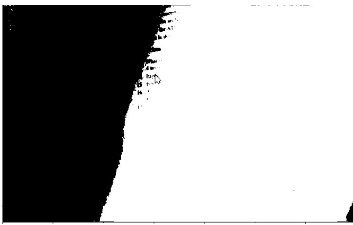
As we can see, we’ve got the lungs completely separated from the rest of the body. Keep in mind this can only be done if images have somewhat of a bimodal histogram.
1.2 Adaptive (local) thresholding
Unlike global thresholding which uses one thresholding value, adaptive thresholding makes use of a unique thresholding value that is based on partitioned sub-images obtained from the whole image. Basically, we divide the image into many small pieces (matrices) and use a certain statistical method, to determine the thresholding value of that sub-image. Let’s now look at this image.
img = cv2.imread('bookthreshold.jpg')
img = cv2.cvtColor(img,cv2.COLOR_BGR2GRAY)
This image won’t have a bimodal histogram because there are many different pixel value groups, simply said there are many shades of gray.
hist,bin_edges = np.histogram(img,bins=256,range=(0,256))
plt.plot(hist)
plt.show()
The histogram is clearly not bimodal, so let’s perform global thresholding and see what happens.
ret,threshold = cv2.threshold(img,130,255,cv2.THRESH_BINARY)
cv2_imshow(threshold)
As we can see, global thresholding clearly doesn’t work here. Now let’s perform adaptive thresholding. We can do that using OpenCV’s function called cv2.adaptiveThreshold. It takes in 6 parameters: image, maximum pixel value, the statistical method of finding threshold value, type of thresholding, size of submatrices (masks), and a constant that helps the algorithm update the thresholding value throughout the process.
threshold2 = cv2.adaptiveThreshold(img,255,cv2.ADAPTIVE_THRESH_MEAN_C,cv2.THRESH_BINARY,13,5)
cv2_imshow(threshold2)
ADAPTIVE_THRESH_MEAN_C means that threshold values will be determined as a mean value of all the pixels in sub-images. You can find the rest of the statistical methods in OpenCV docs. With THRESHOLD_BINARY we’re clarifying that we want a basic binary image as an outcome, meaning pixels higher than their threshold will have the value of 255, and the rest will be set to 0.
Without diving into math, the number 13 determines that the size of the sub-image will be 13×13, all you need to keep in mind is that this number has to be an odd number, and we set a constant to 5. We chose those 2 numbers arbitrarily. The result is as follows:

That looks much better than the global thresholding one. With fine-tuning of the parameters and experimenting with the statistical methods, we could have got an even better image, but this is good enough to show the difference.
2. Edge Detection
Probably one of the most common prerequisites to many problems is finding the edges. Almost every algorithm that is supposed to find some kind of object in the image is based on edge detection. But how is edge detection done? There are plenty of algorithms for that purpose and pretty much all of them have complicated math backgrounds. In this article, we are going to show you how to implement probably the best method for finding all edges in the image.
2.1 Canny Edge Detection
Canny Edge Detection has been one of the most common methods for identifying edges in an image, but also it is one of the most complicated. In this article we’re not going to cover the theoretical background behind Canny Edge Detection, we are just going to focus on its implementation. So let’s dive into it.
import cv2
image = cv2.imread(r'/content/drive/MyDrive/shapessm.jpg')
cv2.imshow(image)
image_edges = cv2.Canny(image,100,200)
cv2.imshow(image_edges)
As you can see Canny implementation in OpenCV is really simple. The canny function takes three arguments: the image we want to detect edges of and two threshold values that we want to separate. You can see that edge detection with OpenCV isn’t hard, but what if we want to get just that CD from the image or maybe that pencil? Edge detection is just the first step in object detection. Now let’s move to the step number two.
3. Line Detection
The task of finding the orientation and location of straight lines in an image is of great importance in image processing. The most commonly used technique when solving this problem is the Hough transform. Hough transformation transposes the image from the spatial domain to another domain where information of interest is represented differently. In this case, we go from spatial to Hough domain.
The backbone of Hough transform is some complex mathematics, and it’s important to note that Hough Transform is not only limited to line detection but any shape that has mathematical parametrization.
3.1 Hough Line Transform
Hough line transform can be done by implementing the cv2.HougLinesP function. The function takes in 5 arguments: Edges of an original image, distance resolution of the accumulator in pixels, distance resolution of the accumulator in radians, and the threshold number of votes inside the function.
Optional parameters are minimum and maximum line length, as well as the gap between the lines. So first we need to perform edge detection on an image.
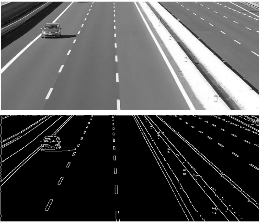
img = cv2.imread('Highway.JPG')
#Converting the image into gray-scale
img = cv2.cvtColor(img,cv2.COLOR_BGR2GRAY)
cv2_imshow(img)
#Finding edges of the image
edge_image = cv2.Canny(img,250,200)
cv2_imshow(edge_image)
Now we want to perform Hough line detection on this image.
lines = cv2.HoughLinesP(edge_image, 1, np.pi/180, 60, minLineLength=10, maxLineGap=250)
#Going through every line we found and drawing it in an image based on starting and ending point
for i in range(2):
  print(lines[i])
#[[  2   1 589   1]]
#[[336   4 542 297]]
This is what the first two lines look like. Each line consists of coordinates of the starting and ending points of a line. The second and third parameters are almost always 1 and Pi/180, and they have to do with Hough transformation math.
The threshold value, minimum line length and maximum line gap have been chosen by experimenting. Now that we’ve got the coordinates of every line, we want to go ahead and draw those lines on our original image.
lines = cv2.HoughLinesP(edge_image, 1, np.pi/180, 60, minLineLength=10, maxLineGap=250)
#Going through every line we found and drawing it in an image based on starting and ending point
for i in range(2):
  print(lines[i])
#[[  2   1 589   1]]
#[[336   4 542 297]]
We’ve successfully identified most of the lines in an image. Let’s now see how we can detect circles using Hough transform.
3.2 Hough Circle Transform
Besides lines, Hough transformation is capable of circle detection. Actually, it’s capable of finding any shapes, if you know their mathematical equations. We encourage you to learn more about this powerful tool in image processing. But if you just need quick circle detection let’s see how it’s done in OpenCV.
import cv2
import numpy as np
from google.colab.patches import cv2_imshow


image = cv2.imread(r'/content/drive/MyDrive/shapessm.jpg')
cv2_imshow(image)

image_edges = cv2.Canny(image, 0,255)
cv2_imshow(image_edges)

circles_img = cv2.HoughCircles(image_edges,cv2.HOUGH_GRADIENT,1,20,
                           param1=50,param2=30,minRadius=40)

circles_img = np.uint16(np.around(circles_img))
for i in circles_img[0,:]:
   image = cv2.circle(image,(i[0],i[1]),i[2],(0,255,0),2)


cv2_imshow(image)
As we can see in the image there is more than one circle-like shape, but we only detected the outer line of that CD that we previously talked about. That has something to do with the parameters of the HoughCircle function and its arguments, so let us try to explain them as simply as possible.
First, as always there is an image on which we want to find circles. The second argument tells us which detection algorithm we want to use, and you should always use cv2.HOUGH_GRADIENT. The third argument has a lot to do with transformation itself, but to make it simple it defines how a full circle line has to be detected. It’s called dp, and the larger it gets, the circle line can be less full and still be detected. Then we have a minimum distance between two detected circles.
Params one and two tell gradient how to detect edges and what is a threshold of a circle-like object, the smaller threshold returns more objects that are not circle-like. Finally, you can set the minimum and maximum radius of the circle you are expecting to detect in pixels.
4. Contour Detection
Contours are defined as the line joining all the points along the boundary of an image that are having the same intensity. Using contour detection, we can detect borders of objects in an image. OpenCV provides the cv2.findContours function that allows us to easily identify all the contours, which is extremely useful in many different tasks. It works the best on binary images, and the function takes in 4 parameters. The image, contours retrieval mode, and the approximation method. Let’s now see how we can perform contour detection.
#Loading the image
img = cv2.imread('/content/drive/MyDrive/shapessm.jpg')
#Converting the image into gray-scale
img = cv2.cvtColor(img,cv2.COLOR_BGR2GRAY)
cv2_imshow(img)
#Output
Now we are going to find edges in this image, using Canny edge detection.
#Finding edges of the image
edge_image = cv2.Canny(img,250,200)
#showing Edged image
cv2_imshow(edge_image)
After we got ourselves this image, we will use OpenCV’s findContours function. Also, we will show how to draw detected contours over the original image using cv2.drawContours function.
# Finding all the lines in an image based on given parameters
contours, hierarchy = cv2.findContours(edge_image,
    cv2.RETR_LIST, cv2.CHAIN_APPROX_SIMPLE)
#Reverting the original image back to BGR so we can draw in colors
img = cv2.cvtColor(img,cv2.COLOR_GRAY2BGR)
#parameter -1 specifies that we want to draw all the contours
cv2.drawContours(img, contours, -1, (0, 255, 0), 3)
cv2_imshow(img)
Let’s now explain the parameters we’ve used. With the contour retrieval type, we have 4 options. Here we used cv2.RETR_LIST which means that the function will retrieve all the possible contours without calculating hierarchy. All the other parameters return the contours in a certain hierarchy, and you can check them in official OpenCV docs. The last parameter represents the approximation method. We have 2 options there.
The first one is cv.CHAIN_APPROX_NONE, which means the function will return all the points in contour and won’t perform any kind of approximation. The second Parameter is cv.CHAIN_APPROX_SIMPLE. Using this parameter the function will approximate keypoint of contours, and provide us with just those points. In the next article, we will see how significant contour detection is, and how we can manipulate these parameters.
Conclusion
In this article, we covered some core principles of image segmentation. Computer vision greatly relies on segmentation, and it is often used as a preprocessing method in some kinds of CNN models. Also, some basic counting applications can be done with some of the algorithms we covered. In the next article, we are going to show you some real-life projects and how you use the image processing knowledge you’ve acquired so far.
Authors

Stefan Nidzovic
Author at Rubik's Code
Stefan Nidzovic is a student at Faculty of Technical Science, at University of Novi Sad. More precisely, department of biomedical engineering, focusing mostly on applying the knowledge of computer vision and machine learning in medicine. He is also a member of “Creative Engineering Center”, where he works on various projects, mostly in computer vision.

Milos Marinkovic
Author at Rubik's Code
Miloš Marinković is a student of Biomedical Engineering, at the Faculty of Technical Sciences, University of Novi Sad. Before he enrolled at the university, Miloš graduated from the gymnasium “Jovan Jovanović Zmaj” in 2019 in Novi Sad. Currently he is a member of “Creative Engineering Center”, where he was involved in a couple of image processing and embedded electronic projects. Also, Miloš works as an intern at BioSense Institute in Novi Sad, on projects which include bioinformatics, DNA sequence analysis and machine learning. When he was younger he was a member of the Serbian judo national team and he holds the black belt in judo.


