Implementing GAN & DCGAN with Python

The code that accompanies this article can be downloaded here.

In the previous article, we started exploring the vast universe of generative algorithms. We started with a gentle introduction to Generative Adversarial Networks or GANs. This major idea, first presented by Ian Goodfellow from the University of Montreal back in 2014, is still regarded as one of the biggest breakthroughs in the field. Facebook’s AI research director, Yann LeCun called this concept “the most interesting idea in the last 10 years in Machine Learning”. Today GANs are even used to generate paintings. Yes, as in art paintings and they are quite pricey.

Generative algorithms, the group of algorithms that GANs are belonging to, are a bit special. We might say that their main goal is completely different from the discriminative algorithms, that we explored in our series on artificial neural networks so far. While discriminative algorithms try to find label based on features, generative algorithms start from the label and generate the features. Mathematically, we can say that they utilize probability p(x|y), where y is given output label and x represents a set of features.

GAN

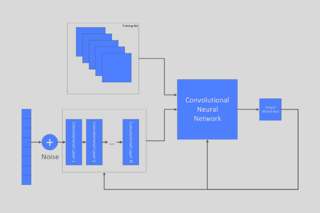
The underlining idea is to use two neural networks instead of one. The training and learning process stay the same and utilize standard techniques (like backpropagation). However, this time we train not one, but two models: a Generative Model (G) and a Discriminative Model (D). Generative Model captures data distribution and uses some sort of noise signal to generates samples and the Discriminative Model is trying to figure out did sample came from the generative model (is it fake) or from the training data (is it real). That looks like something like this:

In a way, we could say that these two models are actually competing against each other. The Generative Model will try to generate data similar to the one from the training set in order to “confuse” the Discriminative Model, while the Discriminative Model will try to improve and recognize is it presented with a fake data. Mathematically, this means they are playing minmax two-player game. This output of the Discriminative Model is then used for backpropagation and for updating both models. You can read more about the main GAN concepts and math behind it here.

Technologies, Dataset and Helpers

Before we dive into the implementation of GAN and later DCGAN, let’s first go through the technologies that we are going to use. We will also say a few words about the used dataset and we will see the implementation of one helper class that will be used for manipulation with image files. In this article, we will use Python 3.6.5 and TensorFlow 1.10.0. A good thing about TensorFlow 1.10.0 is that it has Keras incorporated within it, so we will use that high-level API. In recent announcements of TensorFlow 2.0, it is indicated that contrib module will be completely removed and that Keras will be default high-level API. This seems like a good moment to get familiar with it and use it for implementation. If you need to install TensorFlow follow this article.

Samples from the dataset that is used can be viewed in the image above. It is called Fashion-MNIST dataset and it is similar to the standard MNIST dataset that we used in some of the previous articles. However, instead of handwritten digits, this dataset contains images of clothes. It has a training set of 60,000 samples and testing set of 10,000 images. Like in MNIST dataset, all 28×28 images have been size-normalized and centered. Finally, let’s check out the implementation of the ImageHelper class:

	import os
	import numpy as np
	import imageio
	import matplotlib.pyplot as plt

	class ImageHelper(object):
	def save_image(self, generated, epoch, directory):
	fig, axs = plt.subplots(5, 5)
	count = 0
	for i in range(5):
	for j in range(5):
	axs[i,j].imshow(generated[count, :,:,0], cmap='gray')
	axs[i,j].axis('off')
	count += 1
	fig.savefig("{}/{}.png".format(directory, epoch))
	plt.close()

	def makegif(self, directory):
	filenames = np.sort(os.listdir(directory))
	filenames = [ fnm for fnm in filenames if ".png" in fnm]

	with imageio.get_writer(directory + '/image.gif', mode='I') as writer:
	for filename in filenames:
	image = imageio.imread(directory + filename)
	writer.append_data(image)

view raw image_helper.py hosted with ❤ by GitHub

This class has two functions. The first one, save_image is used to save generated image to the defined file location. The epoch number is used to generate the name of the file. The second function, makegif is used to make .gif file from the images in defined folder. Ok, now we should be up to speed, so we can explore GAN implementation.

Implementation

The implementation of standard Generative Adversarial Network is done in the GAN class. Here it is:

	from __future__ import print_function, division

	import numpy as np
	import pandas as pd
	import matplotlib.pyplot as plt

	# Keras modules
	from tensorflow.keras.layers import Input, Dense, Reshape, Flatten, BatchNormalization, LeakyReLU
	from tensorflow.keras.models import Sequential, Model
	from tensorflow.keras.optimizers import Adam

	class GAN():
	def __init__(self, image_shape, generator_input_dim, image_hepler):
	optimizer = Adam(0.0002, 0.5)

	self._image_helper = image_hepler
	self.img_shape = image_shape
	self.generator_input_dim = generator_input_dim

	# Build models
	self._build_generator_model()
	self._build_and_compile_discriminator_model(optimizer)
	self._build_and_compile_gan(optimizer)

	def train(self, epochs, train_data, batch_size):

	real = np.ones((batch_size, 1))
	fake = np.zeros((batch_size, 1))
	history = []
	for epoch in range(epochs):
	# Train Discriminator
	batch_indexes = np.random.randint(0, train_data.shape[0], batch_size)
	batch = train_data[batch_indexes]
	genenerated = self._predict_noise(batch_size)
	loss_real = self.discriminator_model.train_on_batch(batch, real)
	loss_fake = self.discriminator_model.train_on_batch(genenerated, fake)
	discriminator_loss = 0.5 * np.add(loss_real, loss_fake)

	# Train Generator
	noise = np.random.normal(0, 1, (batch_size, self.generator_input_dim))
	generator_loss = self.gan.train_on_batch(noise, real)

	# Plot the progress
	print ("———————————————————")
	print ("****************Epoch {}*************************".format(epoch))
	print ("Discriminator loss: {}".format(discriminator_loss[0]))
	print ("Generator loss: {}".format(generator_loss))
	print ("———————————————————")

	history.append({"D":discriminator_loss[0],"G":generator_loss})

	# Save images from every hundereth epoch generated images
	if epoch % 100 == 0:
	self._save_images(epoch)

	self._plot_loss(history)
	self._image_helper.makegif("generated/")

	def _build_generator_model(self):
	generator_input = Input(shape=(self.generator_input_dim,))
	generator_seqence = Sequential(
	[Dense(256, input_dim=self.generator_input_dim),
	LeakyReLU(alpha=0.2),
	BatchNormalization(momentum=0.8),
	Dense(512),
	LeakyReLU(alpha=0.2),
	BatchNormalization(momentum=0.8),
	Dense(1024),
	LeakyReLU(alpha=0.2),
	BatchNormalization(momentum=0.8),
	Dense(np.prod(self.img_shape), activation='tanh'),
	Reshape(self.img_shape)])

	generator_output_tensor = generator_seqence(generator_input)
	self.generator_model = Model(generator_input, generator_output_tensor)

	def _build_and_compile_discriminator_model(self, optimizer):
	discriminator_input = Input(shape=self.img_shape)
	discriminator_sequence = Sequential(
	[Flatten(input_shape=self.img_shape),
	Dense(512),
	LeakyReLU(alpha=0.2),
	Dense(256),
	LeakyReLU(alpha=0.2),
	Dense(1, activation='sigmoid')])

	discriminator_tensor = discriminator_sequence(discriminator_input)
	self.discriminator_model = Model(discriminator_input, discriminator_tensor)
	self.discriminator_model.compile(loss='binary_crossentropy',
	optimizer=optimizer,
	metrics=['accuracy'])
	self.discriminator_model.trainable = False

	def _build_and_compile_gan(self, optimizer):
	real_input = Input(shape=(self.generator_input_dim,))
	generator_output = self.generator_model(real_input)
	discriminator_output = self.discriminator_model(generator_output)

	self.gan = Model(real_input, discriminator_output)
	self.gan.compile(loss='binary_crossentropy', optimizer=optimizer)

	def _save_images(self, epoch):
	generated = self._predict_noise(25)
	generated = 0.5 * generated + 0.5
	self._image_helper.save_image(generated, epoch, "generated/")

	def _predict_noise(self, size):
	noise = np.random.normal(0, 1, (size, self.generator_input_dim))
	return self.generator_model.predict(noise)

	def _plot_loss(self, history):
	hist = pd.DataFrame(history)
	plt.figure(figsize=(20,5))
	for colnm in hist.columns:
	plt.plot(hist[colnm],label=colnm)
	plt.legend()
	plt.ylabel("loss")
	plt.xlabel("epochs")
	plt.show()

view raw gan.py hosted with ❤ by GitHub

That is a lot of code, so let’s describe it’s main parts. In the beginning, we import all necessary modules and classes. Keras classes and modules are especially important so we put them in a special section. The constructor of the GAN class is pretty simple and in an essence, it delegates construction of the Generative Model and the Discriminative Model to specialized functions. Apart from that, it initializes optimizer and as you can see Adam optimizer is used.

The fun is happening in the specialized functions: _build_generator_model, _build_and_compile_discriminator_model and _build_and_compile_gan. These functions require our special attention. The first two functions are using Sequential class to create the required model and the third one combines these two models into complete GAN model. Let’s first check out _build_generator_model function:

	def _build_generator_model(self):
	generator_input = Input(shape=(self.generator_input_dim,))
	generator_seqence = Sequential(
	[Dense(256, input_dim=self.generator_input_dim),
	LeakyReLU(alpha=0.2),
	BatchNormalization(momentum=0.8),
	Dense(512),
	LeakyReLU(alpha=0.2),
	BatchNormalization(momentum=0.8),
	Dense(1024),
	LeakyReLU(alpha=0.2),
	BatchNormalization(momentum=0.8),
	Dense(np.prod(self.img_shape), activation='tanh'),
	Reshape(self.img_shape)])

	generator_output_tensor = generator_seqence(generator_input)
	self.generator_model = Model(generator_input, generator_output_tensor)

view raw gan_generator_model.py hosted with ❤ by GitHub

We can see that standard layers were used. Firstly, Input class is used to create an input layer. Than Sequential class is used to describe the rest of the model. Dense class glues LeakyReLU and BatchNormalization layers together. Finally, the tahn and Reshape layers are used to push the output image to output. We already cheated a little bit here by using BatchNormalization and LeakyReLU layers. This is done in order to get better results. Function _build_and_compile_discriminator_model is very similar:

	def _build_and_compile_discriminator_model(self, optimizer):
	discriminator_input = Input(shape=self.img_shape)
	discriminator_sequence = Sequential(
	[Flatten(input_shape=self.img_shape),
	Dense(512),
	LeakyReLU(alpha=0.2),
	Dense(256),
	LeakyReLU(alpha=0.2),
	Dense(1, activation='sigmoid')])

	discriminator_tensor = discriminator_sequence(discriminator_input)
	self.discriminator_model = Model(discriminator_input, discriminator_tensor)
	self.discriminator_model.compile(loss='binary_crossentropy',
	optimizer=optimizer,
	metrics=['accuracy'])
	self.discriminator_model.trainable = False

view raw gan_discriminator_model.py hosted with ❤ by GitHub

Here we build a standard classification neural network with Dense and LeakyReLU classes. In the final layer, we have only one neuron. Basically, the output will tell us was real or fake image sent to the Discriminative Model. It is important to notice that trainable property of this model is set to false. This is done like this because at first, we will train only generator model. Another function, that we need to take look into is train function:

	def train(self, epochs, train_data, batch_size):

	real = np.ones((batch_size, 1))
	fake = np.zeros((batch_size, 1))
	history = []
	for epoch in range(epochs):
	# Train Discriminator
	batch_indexes = np.random.randint(0, train_data.shape[0], batch_size)
	batch = train_data[batch_indexes]
	genenerated = self._predict_noise(batch_size)
	loss_real = self.discriminator_model.train_on_batch(batch, real)
	loss_fake = self.discriminator_model.train_on_batch(genenerated, fake)
	discriminator_loss = 0.5 * np.add(loss_real, loss_fake)

	# Train Generator
	noise = np.random.normal(0, 1, (batch_size, self.generator_input_dim))
	generator_loss = self.gan.train_on_batch(noise, real)

	# Plot the progress
	print ("———————————————————")
	print ("****************Epoch {}*************************".format(epoch))
	print ("Discriminator loss: {}".format(discriminator_loss[0]))
	print ("Generator loss: {}".format(generator_loss))
	print ("———————————————————")

	history.append({"D":discriminator_loss[0],"G":generator_loss})

	# Take a snapshot every 100th epoch
	if epoch % 100 == 0:
	self._save_images(epoch)

	self._plot_loss(history)
	self._image_helper.makegif("generated/")

view raw gan_train.py hosted with ❤ by GitHub

In this function, we first train the discriminator and after that, we train the generator model. We keep the loss in history variable and plot it once the training is done. Apart from that, we take a snapshot of generated images every 100 epochs.

Using GAN class is rather simple. All we have to do is create object of ImageHelper class first and inject it into GAN constructor along with other desired parameters. After that, we can simply call train function:

	import numpy as np
	from keras.datasets import fashion_mnist

	from image_helper import ImageHelper
	from gan import GAN

	(X, _), (_, _) = fashion_mnist.load_data()
	X_train = X / 127.5 – 1.
	X_train = np.expand_dims(X_train, axis=3)

	image_helper = ImageHelper()
	generative_advarsial_network = GAN(X_train[0].shape, 100, image_helper)
	generative_advarsial_network.train(30000, X_train, batch_size=32)

view raw usage_gan.py hosted with ❤ by GitHub

Just one note here. Input data is scaled to -1 to 1 range. This could’ve been done using Sci-Kit Learn or some other library, however since we are familiar with the dataset, we have done it manually.

Results

At the beginning of the training, the Generator Model is very bad, and the only thing it generates is noise:

However, we can see that by the 1000th epoch we already generate more meaningful images. We can already see some contours:

By the 3000th epoch images are looking even better:

After this, however we can see stagnation of the results. Model is improving too slow from this moment on. Take a look at 10000th epoch:

Final epoch gives us these results:

We can see that final results are ok-ish. There are a lot mistakes in the images and the general feel is that this should be better. We will improve these results using DCGAN a little bit later. Just for fun sake, I created an .gif of all these images:

The other fun thing to observe is the loss. Take a look how it oscillates as each model gets better in time:

DCGAN

GANs biggest problem is that they are unstable to train (note the oscilations of the loss). This is due to the fact we train two networks from the same backpropagation. Also, we already know that we have better tools when it comes to image processing and deep learning – Convolutional Neural Networks (CNN). By combining main CNN concepts with GAN ideas, we can improve in this task and generate better images. That is how Deep Convolutional Generative Adversarial Network (DCGAN) were created.

In order to stabilize GANs training, authors of DCGAN proposed several improvements:

Utilizing the convolution layer instead pooling function in the Discriminator model for reducing dimensionality. This way, the network itself will learn how to reduce dimensionality. On the other hand, in the Generator Model, we use deconvolution to upsample dimensions of feature maps.
Adding in the batch normalization. This is used to increase the stability of a neural network. In an essence, batch normalization normalizes the output of a previous layer by subtracting the batch mean and dividing by the batch standard deviation.
Remove fully connected layers from Convolutional Neural Network.
Use Relu and Leaky Relu activation functions.

Implementation

The implementation of DCGAN is done in DCGAN class. The structure of the class is pretty much the same as of GAN class. The only difference are the layers that we use for building our models. Insed of standard layers, like Dense we used convolutional layers, like Conv2D and UpSampling2D. Take a look:

	from __future__ import print_function, division

	import numpy as np
	import pandas as pd
	import matplotlib.pyplot as plt

	# Keras modules
	from tensorflow.keras.layers import Input, Dense, Reshape, Flatten, Dropout, BatchNormalization, Activation, ZeroPadding2D, LeakyReLU, UpSampling2D, Conv2D
	from tensorflow.keras.models import Sequential, Model
	from tensorflow.keras.optimizers import Adam

	class DCGAN():
	def __init__(self, image_shape, generator_input_dim, image_hepler, img_channels):
	optimizer = Adam(0.0002, 0.5)

	self._image_helper = image_hepler
	self.img_shape = image_shape
	self.generator_input_dim = generator_input_dim
	self.channels = img_channels

	# Build models
	self._build_generator_model()
	self._build_and_compile_discriminator_model(optimizer)
	self._build_and_compile_gan(optimizer)

	def train(self, epochs, train_data, batch_size):

	real = np.ones((batch_size, 1))
	fake = np.zeros((batch_size, 1))
	history = []
	for epoch in range(epochs):
	# Train Discriminator
	batch_indexes = np.random.randint(0, train_data.shape[0], batch_size)
	batch = train_data[batch_indexes]
	genenerated = self._predict_noise(batch_size)
	loss_real = self.discriminator_model.train_on_batch(batch, real)
	loss_fake = self.discriminator_model.train_on_batch(genenerated, fake)
	discriminator_loss = 0.5 * np.add(loss_real, loss_fake)

	# Train Generator
	noise = np.random.normal(0, 1, (batch_size, self.generator_input_dim))
	generator_loss = self.gan.train_on_batch(noise, real)

	# Plot the progress
	print ("———————————————————")
	print ("****************Epoch {}*************************".format(epoch))
	print ("Discriminator loss: {}".format(discriminator_loss[0]))
	print ("Generator loss: {}".format(generator_loss))
	print ("———————————————————")

	history.append({"D":discriminator_loss[0],"G":generator_loss})

	# Save images from every hundereth epoch generated images
	if epoch % 100 == 0:
	self._save_images(epoch)

	self._plot_loss(history)
	self._image_helper.makegif("generated-dcgan/")

	def _build_generator_model(self):
	generator_input = Input(shape=(self.generator_input_dim,))
	generator_seqence = Sequential(
	[Dense(128 * 7 * 7, activation="relu", input_dim=self.generator_input_dim),
	Reshape((7, 7, 128)),
	UpSampling2D(),
	Conv2D(128, kernel_size=3, padding="same"),
	BatchNormalization(momentum=0.8),
	Activation("relu"),
	UpSampling2D(),
	Conv2D(64, kernel_size=3, padding="same"),
	BatchNormalization(momentum=0.8),
	Activation("relu"),
	Conv2D(self.channels, kernel_size=3, padding="same"),
	Activation("tanh")])

	generator_output_tensor = generator_seqence(generator_input)
	self.generator_model = Model(generator_input, generator_output_tensor)

	def _build_and_compile_discriminator_model(self, optimizer):
	discriminator_input = Input(shape=self.img_shape)
	discriminator_sequence = Sequential(
	[Conv2D(32, kernel_size=3, strides=2, input_shape=self.img_shape, padding="same"),
	LeakyReLU(alpha=0.2),
	Dropout(0.25),
	Conv2D(64, kernel_size=3, strides=2, padding="same"),
	ZeroPadding2D(padding=((0,1),(0,1))),
	BatchNormalization(momentum=0.8),
	LeakyReLU(alpha=0.2),
	Dropout(0.25),
	Conv2D(128, kernel_size=3, strides=2, padding="same"),
	BatchNormalization(momentum=0.8),
	LeakyReLU(alpha=0.2),
	Dropout(0.25),
	Conv2D(256, kernel_size=3, strides=2, padding="same"),
	BatchNormalization(momentum=0.8),
	LeakyReLU(alpha=0.2),
	Dropout(0.25),
	Flatten(),
	Dense(1, activation='sigmoid')])

	discriminator_tensor = discriminator_sequence(discriminator_input)
	self.discriminator_model = Model(discriminator_input, discriminator_tensor)
	self.discriminator_model.compile(loss='binary_crossentropy',
	optimizer=optimizer,
	metrics=['accuracy'])
	self.discriminator_model.trainable = False

	def _build_and_compile_gan(self, optimizer):
	real_input = Input(shape=(self.generator_input_dim,))
	generator_output = self.generator_model(real_input)
	discriminator_output = self.discriminator_model(generator_output)

	self.gan = Model(real_input, discriminator_output)
	self.gan.compile(loss='binary_crossentropy', optimizer=optimizer)

	def _save_images(self, epoch):
	generated = self._predict_noise(25)
	generated = 0.5 * generated + 0.5
	self._image_helper.save_image(generated, epoch, "generated-dcgan/")

	def _predict_noise(self, size):
	noise = np.random.normal(0, 1, (size, self.generator_input_dim))
	return self.generator_model.predict(noise)

	def _plot_loss(self, history):
	hist = pd.DataFrame(history)
	plt.figure(figsize=(20,5))
	for colnm in hist.columns:
	plt.plot(hist[colnm],label=colnm)
	plt.legend()
	plt.ylabel("loss")
	plt.xlabel("epochs")
	plt.show()

view raw dcgan.py hosted with ❤ by GitHub

Because we were able to keep the same API, the usage of this class is the same as well. The only difference is that training is done in 20000 epochs, not in 30000 like we did for GAN. The reason for that is that training fro DCGAN lasts much longer. Without further ado, here is how DCGAN class is used:

	import numpy as np
	from keras.datasets import fashion_mnist

	from image_helper import ImageHelper
	from dcgan import DCGAN


	(X, _), (_, _) = fashion_mnist.load_data()
	X_train = X / 127.5 – 1.
	X_train = np.expand_dims(X_train, axis=3)

	image_helper = ImageHelper()
	generative_advarsial_network = DCGAN(X_train[0].shape, 100, image_helper, 1)
	generative_advarsial_network.train(20000, X_train, batch_size=32)

view raw usage_dcgan.py hosted with ❤ by GitHub

Results

Here we expect better results, and indeed we got them. In the beginning, we had just noise, just like with GAN:

By the 1000th epoch, we got something more concrete. The result is better than GAN’s 1000th epoch as well:

The trend continued in 3000th epoch:

And in 10000th epoch:

Finally, in the 20000th epoch we got something like this:

Conclusion

In this article we had a chance to go deeper into the GAN and DCGAN structure. We had a chance to use theoretical knowledge from the previous article and implement these architectures using Python and TensorFlow. In the end, we managed to generate pretty good images using DCGAN, but we definitely can do better. In next article, we will try to improve these results even more using some more advanced GAN architectures.

Thank you for reading!

This article is a part of Artificial Neural Networks Series, which you can check out here.

Read more posts from the author at Rubik’s Code.