Introduction to Generative Adversarial Networks (GANs)

Deep Learning zoo is getting bigger by the day. This is probably due to the fact that we are “crossing the chasm” with this technology and that we are entering “early majority” phase. Simply put, people find more and more ways to use deep learning concepts and come up with different forms of neural networks. So far in our journey through this intriguing world, we covered many topics, different architectures of neural networks and types of learning. However, we explored just discriminative algorithms and not the generative ones (more on that later) and these types of algorithms are some of the most interesting cases that could be found in this neural networks universe.

One of those interesting cases is Generative Adversarial Network or GAN. This architecture was first presented in the paper by Ian Goodfellow from the University of Montreal back in 2014. and they took the world by storm. Even Yann LeCun,  Facebook’s AI research director, called them “the most interesting idea in the last 10 years in Machine Learning”. Using this concept people started creating surreal combinations of Kubrick and Picasso and even sold art created by GANs for a lot of money (and I mean a lot of money).

Apparently, before we dive into all the details of this concept, we need to discuss generative algorithms for a little bit. Different kinds of chatbots, speech2text and text2speech, image captioning and quality enhancements and other cool applications have some kind of generative model under the hood. As mentioned, in our series we covered only discriminative algorithms.

These algorithms are used for classification, and they do so by using labels. For example, we were able to predict a type of Iris Flower in one of our previous articles. There we had to recognize three different classes of Iris plant: Iris setosa, Iris virginica, and Iris versicolor. These three class names are actualy labels and classification is done by mapping certain features to those labels. Mathematically, we can say that they use the probability that given certain features x we will get label y – p(y|x).

Generative algorithms are a bit different. They start from the label and generate the features. In our example, we would say “Ok, let’s create features that will give Iris setosa label as output”. Essentially they are the opposite of the discriminative algorithms. Again, mathematically, they use probability that given certain output label y we get features x – p(x|y). They can be used as classifiers as well, but that is a story for another time.

 Player 2 has Entered the Game

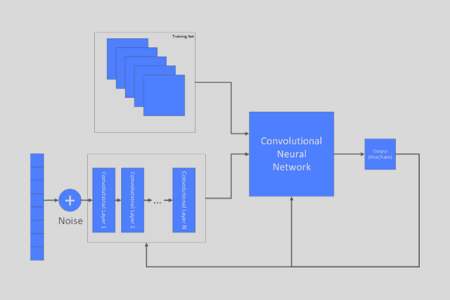
The big secret of GAN is that underneath they don’t have just one neural network, but two neural networks. The learning process uses all standard techniques, like backpropagation, but this time we train two models: a Generative Model (G) and a Discriminative Model (D). The first one captures data distribution and generates samples and the second one is calculating the probability that a presented sample came from the training data and not from the generative model.

This means that these two networks are competing against each other. The Generative Model will try to generate samples for which Discriminative Model will conclude that they are coming from the training dataset. Essentially, during the learning process, the Generative Model will try to maximize the probability of the Discriminative Model creating a mistake, which corresponds to minmax two-player game (more on that later). The whole thing can be represented using the image below.

To sum it up, the Discriminative Model gets samples from both training set and from the Generative Model and as an output provides an information do we have the fake sample (the one that is coming from the Generative Model) or the real one (the one that is coming from the training set). This output is then used for backpropagation and for updating both models. The Generative Model, on the other hand, uses random noised data as an input, and as an output provides a sample for the Discriminative Model. The final result of this competition is that the Generative Model will be able to create real looking samples. 

Math Behind the Magic

As mentioned, GANs are using a concept of minmax two players game. This is a decision rule used in game theory and statistics for minimizing the possible loss for a worst case scenario (maximum loss). How does that look in our architecture? Well, we can say that D(x) represents the probability that sample x came from the training set rather than the Generative Model. We train the Discriminative Model to maximize the probability of assigning the correct label to both types of samples. At the same time, we train the Generative Model to minimize log(1 − D(G(z))), where z is an input into the Generative Model. The whole thing can be described with the function: 

The Discriminative Model tries to maximize the function above. This means that we can perform gradient ascent on the function. On the other hand, the Generative Model tries to minimize the same function, which means we can perform gradient descent on the function. The network is then trained by alternating between gradient ascent and descent. To put it matematically, the Disciminative Model is updated using:

, and the Generative Model is updated using:

This is the theory behind it. However, in the lab during the experiment, we got different results. The problem was that in the beginning the Generative Model will produce samples that are obviousl fake, and this can cause stagnation of the function log(1 − D(G(z))). It is observed that better results are achieved once we use log(D(G(z))).

Different Architectures

Since we train two networks from the same backpropagation, GANs are unstable to train. Also, the idea was to use these networks for generating images and they don’t achieve good results in that area. That is why another solution evolved from this concept – Deep Convolutional Generative Adversarial Network (DCGAN). As you can imagine this architecture combines the concepts from Convolutional Neural Networks with just explained GAN concepts. Meaning, it uses convolutional stride and transposed convolution for the downsampling and the upsampling. Using this approach we get better results as we will see in future articles. This arhitecture looks something like this:

To further improve these results we can use Autoencoders. We already know that autoencoders are not good for image compression, but we know they are good for dimensionality reduction. They fit data into the Gaussian distribution, but eventually, they produce blurry images. So, how we can utilize them here. The truth is that we are using a special type of Autoencoders – Variational Autoencoders (VAE). This type of autoencoder has a structure that resembles classical autoencoder, ie. it consists of an encoder, decoder and a loss function. However, after encoder part of the network, we define two layers. One that defines mean deviation and the other that represents standard deviation. From this we get needed latent vector (it is called latent because using it we can not figure out the parameters of the model that produced it).

So, how this fits into our GAN story? Well, as it turns out the combination of Variational Autoencoders and Deep Convolutional Generative Adversarial Network gives fantastic results. In this arhitectural combination the Generative Model is acting as a decoder part of the network as well. The whole thing looks something like this:

Conclusion

In this article, we scratched the interesting topic of Generative Adversarial Networks. In a way, they changed the way we are using neural networks, not just for solving classification and regression problems. Now we are able to generate data using them as well. Their fairly similar approach is giving us many possibilities and as we saw the opportunity to combine different types of neural networks together. In a next article, we will use the knowlege we gathered here and create concrete implementation of such network.

Thank you for reading!

---

This article is a part of  Artificial Neural Networks Series, which you can check out here.

---

Read more posts from the author at Rubik’s Code.

---