

In the previous couple of articles, we explored reinforcement learning ecosystem, how it can be described and how it functions. Reinforcement learning is a type of learning that is different from supervised and unsupervised learning. Unlike the mentioned approaches, reinforcement learning uses interaction, which makes it “the third paradigm of machine learning“. Main reinforcement learning elements are learning agent and environment. These two elements are in constant interaction. Learning agent has a certain goal it wants to accomplish within the environment. In its quest, learning agent performs actions which are defined by the environment. Essentially, environment has set of states and for each state there is certain number of actions defined. By performing actions, learning agent changes the state of the environment and for each action it gets certain reward. The goal of the agent is to maximize that reward.
Eager to learn how to build Deep Learning systems using Tensorflow 2 and Python? Get the ebook here!

This ecosystem is usually formalized with Markov Decision Processes (MDPs). MDP is essentially a tuple containing four elements:
- S – Set of states. At each time step t, the agent gets the environment’s state – St, where St ∈ S.
- A – Set of actions that the agent can take.
- Pa – Probability that action in some state s will result in the time step t, will result in the state s’ in the time step t+1.
- Ra – Or Ra(s, s’), represents expected reward received after going from state s to the state s’, as a result of action a.
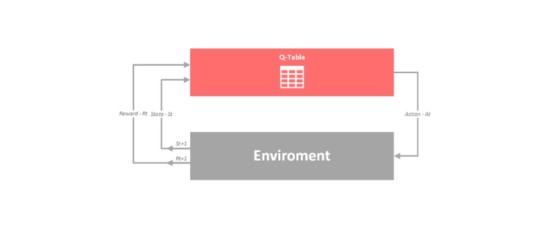
MDPs are often visualized using image below:

Thus far on our site we focused on the most popular algorithms of reinforcement learning – Q-Learning. This algorithm is quite clever. How so? Well, it estimates the value of taking action a in state s under policy π, i.e. Q-Value of each action in each state. Decisions are based on estimations of state-action pairs. It is defined by the formula:

A Q-Value for a particular state-action combination can be observed as the quality of an action taken from that state. All these Q-Values are stored inside of the Q-Table, which is just the matrix with the rows for states and the columns for actions. This table is updated by the agent. For more information about Q-Learning check out this article.
However, this algorithm has one major flaw, which makes it perform bad in highly stochastic environments. That is the most integral part of the formula – maxQ(St+1, a). This part of the formula is used to calculate Q-value of the current time step is based on the Q-value of the time step from the future. How that works? First, we initialize Q-Values for states St and St+1 to some random values. Then, during the training process we update Q-Value in the state St based on Q-Value in the state St+1. As it turns out, max operator causes overestimation of Q-Values. In the previous article, we explored the problem that we are facing with Q-learning overestimation and how this can be solved with Double Q-Learning. Let’s empirically prove that.
Q-Learning Problem

So, we already explained the core of the problem. Q-Learning overestimates Q-Values in certain environments, which can lead to choosing wrong actions and building wrong policies. To be more precise, let’s explore environment which can be represented with the image below:
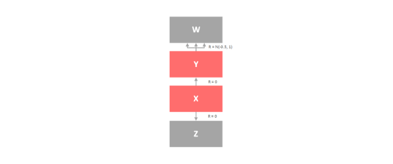
This is one simple environment with 4 states: X, Y, Z and W. X is starting state , while states Z and W are terminal. There are two actions that agent can take in state X – UP and DOWN. Reward fro taking these actions is 0. The interesting part is the set of actions from state Y to W. The reward for this set of actions follows normal distribution with mean -0.5 and standard deviation 1. This means that after a large number of iterations reward will be negative:
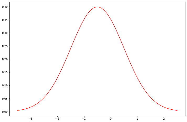
This in turn means that our learning agent should never pick the action UP from the state X in the first place, if it wants to minimize the loss, i.e. the goal of the agent would actually be to get reward 0, or the least negative value. This is where Q-Learning has problems. Because we have that specific distribution of reward learning agent can be fooled that it should take action UP in the state X. In a nutshell, max operator updates the Q-Value, which could be positive for this action, learning agent takes this action as valid option. Q-Value is overestimated! Before we proceed with the implementation, let’s import necessary libraries and define some globals:
import numpy as np
import random
from IPython.display import clear_output
import gym
import matplotlib.pyplot as plt

# Globals
ALPHA = 0.1
GAMMA = 0.6
EPSILON = 0.05
As the first step of this experiment we implement simple environment:
class MDP():
    def __init__(self, action_tree=9):
        # Actions
        self.down, self.up = 0, 1

        # States and posible actions
        self.state_actions = {
            'X': [self.down, self.up],
            'Y': [i for i in range(action_tree)],
            'W': [self.down],
            'Z': [self.up] }

        # Transitions
        self.transitions = {
            'X': {self.down: 'Z',
                  self.up: 'Y'},
            'Y': {a: 'W' for a in range(action_tree)},
            'W': {self.down: 'Done'},
            'Z': {self.up: 'Done'}
        }

        self.states_space = 4
        self.action_space = action_tree
        self.state = 'X'

    def _get_reward(self):
        return np.random.normal(-0.5, 1) if self.state == 'W' else 0

    def _is_terminated_state(self):
        return True if self.state == 'W' or self.state == 'Z' else False

    def reset(self):
        self.state = 'X'
        return self.state

    def step(self, action):
        self.state = self.transitions[self.state][action]
        return self.state, self._get_reward(), self._is_terminated_state(), None

    def available_actions(self, state):
        return self.state_actions[state]

    def random_action(self):
        return np.random.choice(self.available_actions(self.state))

mdp_enviroment = MDP()
In the constructor of this class we initialize actions and dictionary that represents states and possible actions in each state. We also create dictionary that defines transitions, i.e. we define which other states are available from some state. Finally, we initialize starting state to X. We have several functions in this class:
- _get_reward – Internal function used to return reward for certain action. In general, only reward is not zero only when we end up in state W.
- _is_terminated_state – Checks weather state is terminal.
- reset – Resets state of the environment to X.
- step – Performs an action.
- available_actions – Returns available actions for provided state.
- random_action – Takes random action.
During the implementation of this environment, we tried to follow Open AI Gym API as much as we could, so we should have fewer changes later on when we decide to switch to Open AI Gym. Don’t forget to create an instance of this class.
Ok, let’s now observe Q-Learning function for this environment:
def mdp_q_learning(enviroment, num_of_tests = 10000, num_of_episodes=300):

    num_of_ups = np.zeros(num_of_episodes)

    for _ in range(num_of_tests):

        # Initialize Q-table
        q_table = {state: np.zeros(9) for state in mdp_enviroment.state_actions.keys()}
        rewards = np.zeros(num_of_episodes)

        for episode in range(0, num_of_episodes):
            # Reset the enviroment
            state = enviroment.reset()

            # Initialize variables
            terminated = False

            while not terminated:
                # Pick action a....
                if np.random.rand() < EPSILON:
                    action = enviroment.random_action()
                else:
                    available_actions = enviroment.available_actions(enviroment.state)
                    state_actions = q_table[state][available_actions]
                    max_q = np.where(np.max(state_actions) == state_actions)[0]
                    action = np.random.choice(max_q)

                # ...and get r and s'
                next_state, reward, terminated, _ = enviroment.step(action)

                # 'up's from state 'X'
                if state == 'X' and action == 1:
                    num_of_ups[episode] += 1

                # Update Q-Table
                max_value = np.max(q_table[next_state])
                q_table[state][action] += ALPHA *
                     (reward + GAMMA * max_value - q_table[state][action])
                state = next_state
                rewards[episode] += reward

    return rewards, q_table, num_of_ups
Function mdp_q_learning implements Q-Learning algorithm:
- Initialize all Q-Values in the Q-Table arbitrary, and the Q value of terminal-state to 0:
Q(s, a) = n, ∀s ∈ S, ∀a ∈ A(s)
Q(terminal-state, ·) = 0 - Repeat for each episode
- Repeat until terminal state is reached
- Pick the action a, from the set of actions defined for that state A(s) defined by the policy π.
- Perform action a
- Observe reward R and the next state s’
- For all possible actions from the state s’ select the one with the highest Q-Value – a’.
- Update value for the state using the formula:
Q(s, a) ← Q(s, a) + α [R + γQ(s’, a’) − Q(s, a)] - s = s’
- Repeat until terminal state is reached
Notice that in this function we count number of times algorithm picked action UP from state X. We returned this value along with the reward so we can plot them:
q_reward, q_table, num_of_ups = mdp_q_learning(mdp_enviroment)

plt.figure(figsize=(15,8))
plt.plot(num_of_ups/10000*100, label='UPs in X', color='#FF171A')
plt.plot(q_reward, color='#6C5F66', label='Reward')
plt.legend()
plt.ylabel('Percentage of UPs in state X')
plt.xlabel('Episodes')
plt.title(r'Q-Learning')
plt.show()
We plotted how many times action UP was chosen in the state X in percents:

We can see that in the beginning Q-learning, because of it’s nature, picked up action UP from the state X quite often. During this period reward was even positive for a couple of episodes. However, when that peak passed we can see that reward stabilized to 0 (mostly). Can this initial time for wrong decisions be improved with Double Q-Learning?
Double Q-Learning

In the previous article we explored Double Q-Learning in detail, so here we will just recap the main points. Double Q-Learning proposes that instead of using just one Q-Value for each state-action pair, we should use two values – QA and QB. This algorithm focuses on finding action a* that maximizes QA in the state next state s’ – (Q(s’, a*) = max Q(s’, a)). Then it uses this action to get the value of second Q-Value – QB(s’, a*). Finally it uses QB(s’, a*) in order to update QA(s, a):

This is done the other way around too for QB. Action b* that maximizes QB in the state next state s’ – (Q(s’, b*) = max Q(s’, b)). This action is used to get the value of another Q-Value – QA(s’, b*). In the end, QB(s, a) is updated with QA(s’, b*).
If we brake it down into steps that looks something like this:
- Initialize all QA, QB and starting state – s
- Repeat
- Pick the action a and based on QA(s, •) and QB(s, •) get r and s’
- Update(A) or Update(B) (pick at random)
- If Update(A)
- Pick the action a* = argmax QA(s’, a)
- Update QA
QA(s, a) ← QA(s, a) + α [R + γQB(s’, a*) − QA(s, a)]
- IfUpdate(B)
- Pick the action b* = argmax QB(s’, a)
- Update QB
QB(s, a) ← QB(s, a) + α [R + γQA(s’, b*) − QB(s, a)]
- s ← s’
- Until End
Implementation of such algorithm in Python for the environment we created looks like this:
def mdp_double_q_learning(enviroment, num_of_tests = 10000, num_of_episodes=300):

    num_of_ups = np.zeros(num_of_episodes)

    for _ in range(num_of_tests):

        # Initialize Q-table
        q_a_table = {state: np.zeros(9) for state in mdp_enviroment.state_actions.keys()}
        q_b_table = {state: np.zeros(9) for state in mdp_enviroment.state_actions.keys()}
        rewards = np.zeros(num_of_episodes)

        for episode in range(0, num_of_episodes):
            # Reset the enviroment
            state = enviroment.reset()

            # Initialize variables
            terminated = False

            while not terminated:
                # Pick action a....
                if np.random.rand() < EPSILON:
                    action = enviroment.random_action()
                else:
                    q_table = q_a_table[state][enviroment.available_actions(enviroment.state)] + \
                        q_b_table[state][enviroment.available_actions(enviroment.state)]
                    max_q = np.where(np.max(q_table) == q_table)[0]
                    action = np.random.choice(max_q)

                # ...and get r and s'
                next_state, reward, terminated, _ = enviroment.step(action)

                # 'up's from state 'X'
                if state == 'X' and action == 1:
                    num_of_ups[episode] += 1

                # Update(A) or Update (B)
                if np.random.rand() < 0.5:
                    # If Update(A)
                    q_a_table[state][action] += ALPHA * (reward + GAMMA * q_b_table[next_state][np.argmax(q_a_table[next_state])] - q_a_table[state][action])

                else:
                    # If Update(B)
                    q_b_table[state][action] = ALPHA * (reward + GAMMA * q_a_table[next_state][np.argmax(q_b_table[next_state])] - q_b_table[state][action])


                state = next_state
                rewards[episode] += reward

    return rewards, q_a_table, q_b_table, num_of_ups
We run it on the instance of the environment like this:
dq_reward, _, _, dq_num_of_ups = mdp_double_q_learning(mdp_enviroment)
Once again we count number of times algorithm picked action UP from state X. Double Q-Learning algorithm figures out the trap much faster:
plt.figure(figsize=(15,8))
plt.plot(dq_num_of_ups/10000*100, label='UPs in X', color='#FF171A')
plt.plot(dq_reward, color='#6C5F66', label='Reward')
plt.legend()
plt.ylabel('Percentage of UPs in state X')
plt.xlabel('Episodes')
plt.title(r'Double Q-Learning')
plt.show()
Observe the plot:

And check it out what it looks like when we put results of both algorithm on the same plot:
plt.figure(figsize=(15,8))
plt.plot(dq_num_of_ups/10000*100, label='Double Q-learning', color='g')
plt.plot(num_of_ups/10000*100, label='Q-learning', color='#FF171A')
plt.legend()
plt.ylabel('Percentage of UPs in state X')
plt.xlabel('Episodes')
plt.title(r'Double Q-Learning vs. Q-Learning')
plt.show()
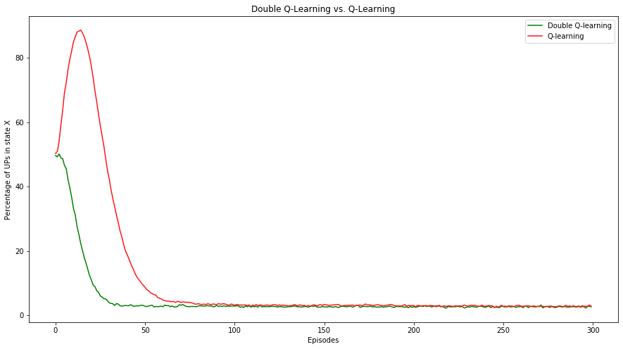
We might say that Double Q-Learning learned optimal policy in half of the training time. Finally if we print out the cumulative reward so we can see who perform better:
height = [dq_reqard_sum, q_reqard_sum]
bars = ('Double Q-Learning', 'Q-Learning')
y_pos = np.arange(len(bars))
plt.bar(y_pos, height, color=('g', '#FF171A'))
plt.xticks(y_pos, bars)
plt.show()
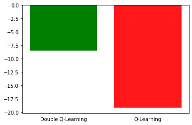
We can see that Double Q-Learning got ~2.5 times better results than vanilla Q-Learning.
Working with Open AI Gym

Ok, we saw what happens when we use two algorithms on stochastic environment. Let’s check what happens when we use these algorithms on Open AI Gym environments. For this experiment we use the environment Taxi-V2. This is relatively simple environment. The environment has 4 locations (states) the agent’s goal is to pick up the passenger at one location and drop him off in another. The agent can perform 6 actions (south, north, west, east, pickup, drop-off). More info about the environment can be found here.

First we need to load the environment:
enviroment = gym.make("Taxi-v2").env
enviroment.render()

print('Number of states: {}'.format(enviroment.observation_space.n))
print('Number of actions: {}'.format(enviroment.action_space.n))
+---------+
|R: | : :G|
| : : : : |
| : : : : |
| | : | : |
|Y| : |B: |
+---------+

Number of states: 500
Number of actions: 6
Then we need to modify Q-Learning and Double Q-Learning functions so they are now applicable to this API. Changes are minimal, but crucial:
def q_learning(enviroment, num_states, num_actions, num_of_episodes=1000):

    # Initialize Q-table
    q_table = np.zeros((enviroment.observation_space.n, enviroment.action_space.n))
    rewards = np.zeros(num_of_episodes)

    for episode in range(0, num_of_episodes):
        # Reset the enviroment
        state = enviroment.reset()

        # Initialize variables
        terminated = False

        while not terminated:
            # Pick action a....
            if np.random.rand() < EPSILON:
                action = enviroment.action_space.sample()
            else:
                max_q = np.where(np.max(q_table[state]) == q_table[state])[0]
                action = np.random.choice(max_q)

            # ...and get r and s'
            next_state, reward, terminated, _ = enviroment.step(action)

            # Update Q-Table
            q_table[state, action] += ALPHA * (reward + GAMMA * np.max(q_table[next_state]) - q_table[state, action])
            state = next_state
            rewards[episode] += reward

    return rewards, q_table
def double_q_learning(enviroment, num_of_episodes=1000):

    q_a_table = np.zeros([enviroment.observation_space.n, enviroment.action_space.n])
    q_b_table = np.zeros([enviroment.observation_space.n, enviroment.action_space.n])
    rewards = np.zeros(num_of_episodes)

    for episode in range(0, num_of_episodes):
        # Reset the enviroment
        state = enviroment.reset()

        # Initialize variables
        terminated = False

        while not terminated:

            # Pick action a....
            if np.random.rand() < EPSILON:
                action = enviroment.action_space.sample()
            else:
                q_table = q_a_table[state] + q_b_table[state]
                max_q = np.where(np.max(q_table) == q_table)[0]
                action = np.random.choice(max_q)

            # ...and get r and s'
            next_state, reward, terminated, _ = enviroment.step(action)

            # Update(A) or Update (B)
            if np.random.rand() < 0.5:
                # If Update(A)
                q_a_table[state, action] += ALPHA * (reward + GAMMA * q_b_table[next_state, np.argmax(q_a_table[next_state])] - q_a_table[state, action])

            else:
                # If Update(B)
                q_b_table[state, action] = ALPHA * (reward + GAMMA * q_a_table[next_state, np.argmax(q_b_table[next_state])] - q_b_table[state, action])

            state = next_state
            rewards[episode] += reward

    return rewards, q_a_table, q_b_table
Finally we can run both functions:
q_reward, q_table = q_learning(enviroment, observation_space, action_space)
dq_reward, q_a_table, q_b_table = double_q_learning(enviroment)
Once they are finished, we can plot out the reward of each algorithm:

What we can notice in this situation is that overall Q-Learning performed better than Double Q-Learning. Even though this might seem strange, it is actually expected to happen. The vanilla Q-Learning learns only one Q-Table and the Double Q-learning must learn two Q-Tables. In essence, Double Q-Learning is less sample efficient, but it provides a better policy.
Conclusion
In this article, we could see how to implement Double Q-Learning algorithm and how to compare it with vanilla Q-Learning. We could see that this algorithm comes up with the better policy. In the next article, we will involve neural networks in the whole story and build so called Deep Double-Q Learning or Double DQN. Stay tuned 🙂
Thank you for reading!
Rubik’s Code is a boutique data science and software service company with more than 10 years of experience in Machine Learning, Artificial Intelligence & Software development. Find out more about the services we provide here.
Eager to learn how to build Deep Learning systems using Tensorflow 2 and Python? Get our ‘Deep Learning for Programmers‘ ebook here!
Read our blog posts here.


Trackbacks/Pingbacks