The code that accompanies this article can be found here.
In a previous couple of articles, we explored some basic machine learning algorithms. Thus far we covered some simple regression algorithms, classification algorithms and algorithms that can be used for both types of problems. We explored algorithms like SVM, Decision Trees and Random Forest.
Apart from that, we dipped our toes in unsupervised learning, saw how we can use this type of learning for clustering and learned about several clustering techniques. In all these articles, we used Python for “from the scratch” implementations and libraries like TensorFlow, Pytorch and SciKit Learn. Also, we used optimization techniques such as Gradient Descent.
Are you afraid that AI might take your job? Make sure you are the one who is building it.
STAY RELEVANT IN THE RISING AI INDUSTRY! 🖖
In this article, we focus on machine learning algorithm performance and its improvement. We explore terms such as bias and variance, and how to balance them in order to achieve better performance. We learn about overfitting and underfitting, ways to avoid them and improve machine learning efficiency with regularization techniques such as Lasso and Ridge.
Dataset and Prerequisites
Data that we use in this article is the famous Boston Housing Dataset. This dataset is composed 14 features and contains information collected by the U.S Census Service concerning housing in the area of Boston Mass. It is a small dataset with only 506 samples.

For the purpose of this article, make sure that you have installed the following Python libraries:
- NumPy – Follow this guide if you need help with installation.
- SciKit Learn – Follow this guide if you need help with installation.
Once installed make sure that you have imported all the necessary modules that are used in this tutorial.
import pandas as pd
import numpy as np
import matplotlib.pyplot as plt

from sklearn.model_selection import train_test_split
from sklearn.metrics import mean_squared_error
from sklearn.linear_model import Lasso, Ridge, ElasticNet, SGDRegressor, LinearRegression
from sklearn.preprocessing import StandardScaler
from sklearn.pipeline import make_pipeline
from sklearn.base import clone
Apart from that, it would be good to be at least familiar with the basics of linear algebra, calculus and probability.
Bias and Variance
When we are talking about the performance of the machine learning model, we always talk about some form of accuracy. We want our model to produce accurate predictions, that is why we do all this, right? During the training process of any machine learning model we try to find the optimal function that will be able to best describe output values, ie. we try to optimize function f(X):

During the training process, we calculate how well the model performs and modify parameters of the f(X) so our result is closer to the real values of Y. While we are doing that we calculate the error of our model. We put in the sample, calculate the error based on the real Y value and modify the parameters of the f(X). The error produced this way is called reducible error because it can be minimized and even completely removed (not a good idea btw). The other part of the equation from above is e – irreducible error.
This error comes from the fact that no matter how good our machine learning model is, X is not carrying all the information that we need to predict Y in every possible scenario. Our model is an approximation, after all, thus it will not be 100% accurate. As George Box said, “All models are wrong, but some are useful”. Essentially, all we can do is optimize parameters of f(X) and get the best possible approximation, ie. we always try to optimize reducible error, because there is nothing we can do about the irreducible error.

This leads us to use different functions for f(X). Sometimes, as we were able to see they are quite easy, understandable and produce a model that is easy to interpret. For example, multiple linear regression output value Y as a combination of features of X:

When we get values of parameters, we can say how each feature affects the final result. Like a recipe. However, if this model doesn’t provide good enough results, we might want to use some other function, something that will better fit the data. So, we go and use more complex functions, like polynomial linear regression. This gives us better results, but it is more complex and harder to explain. Also, the complex model might make assumptions that are not really correct, or pick up some patterns that are caused by random chance rather than by true properties and make bad predictions on test/real data.

Here we can observe two possibilities, either we choose a model that is not that complex and get bad results on training data, or choose a complex model that might give bad results on test data. The first case is called underfitting – the inability of the machine learning model to predict well the labels of the data it was trained on. As mentioned, this is happening when we are using a model that is not complex enough, but it can happen if the features in the dataset are not informative enough.
The other case is overfitting – the model predicts very well on the training data but makes a lot of errors when applied to samples that were not processed by it during either the training phase. These models have bad performance in the testing phase or during production. This happens if the model is to complex for a data or/and we have too many features but a small number of samples in the dataset.

In order to avoid both underfitting and overfitting, we need to represent reducible error as a sum of bias and variance. This means that models complete generalization error can be represented as:

Bias is the error that is introduced when we are approximating a real-life problem, which may be extremely complicated, with a simple model. This of course leads to underfitting, and we say that such models have a high bias. However, when a model shows high sensitivity to small variations in training data, we say that it has high-variance. In essence, the variance can be defined as the amount by which your estimate of f(X) would change if we estimated it using a different training data set. High-variance leads to overfitting and it is the biggest problem with flexible (and complex) models.

In literature, this problem is often called a bias-variance tradeoff. We can define a rule like this – as a machine learning model tries to match data points more accurately or when a more complex method is used, the bias reduces, but variance increases. In order to minimize the generalization error, we need to select a machine learning model that simultaneously achieves low variance and low bias.
Regularization
One way to minimize the chance of overfitting is by using regularization. In general, this is an umbrella term that refers to different techniques that force the learning algorithm to build a less complex model by constraining it in one way or another. The idea is that if the model has less freedom the harder it will be for it to overfit the data. In practice, this often leads to higher bias but reduces the variance. Some of the most popular regularization techniques constrain the model’s weights/coefficients. In this article, we explore three such methods – Lasso, Ridge and ElasticNet. Also, we explore the Early Stopping Technique, which is a different regularization technique, but more on that later. Before going into more details of each technique, let’s first load the data and prepare it for processing.
Data Preparation
Boston Housing Dataset is located in the .csv file, so let’s load it:
data = pd.read_csv('./data/boston_housing.csv')
data.head()
In this article, we use only the ‘lstat’ feature as input and the ‘medv‘ feature as an output. Here is how that looks like:
data = data.dropna()

X = data['lstat'].values
X = X.reshape(-1, 1)

y = data['medv'].values

X_train, X_test, y_train, y_test = train_test_split(X, y, test_size=0.2, random_state=33)

plt.scatter(x = X, y = y, color='orange')
plt.show()
In one of the previous articles, we applied linear regression to this data and here is what we got:
linear_reg = make_pipeline(StandardScaler(), LinearRegression())
linear_reg.fit(X_train, y_train)
linear_reg_predictions = linear_reg.predict(X_test)

pd.DataFrame({
    'Actual Value': y_test,
    'Ridge Prediction': linear_reg_predictions,
})
Here is what that looks like when we plot it out:

Ridge Regression
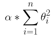
Ridge Regression, also known as Tikhonov regularization or L2 norm, is a modified version of Linear Regression where the cost function is modified by adding the “shrinkage quality“. In essence, the regularization term is added to the cost function:

This is done during the training process (not during testing, just during training). This forces the machine learning algorithm not only to better fit data but also to keep the model as simple as possible because the linear regression coefficients are optimized in a way to minimize this modified function.

Notice that this additional term prevents coefficients from rising too high. Apart from that, notice that α drives the level of regularization and that we need to be careful when we are picking it. If it is close to 0, the regularization has no effect, but as α→∞ regression, coefficients are getting closer to 0. So, if we use MSE (mean squared error) as a loss function, the Ridge regression cost function would be:

Note that the bias term θ0 is not regularized, because the sum starts from i=1, not from i=0. In essence, the regularization term can be defined with the formula:

where w is the vector of feature coefficients (from θ1 to θn) and ∥ · ∥2 represents the L2 norm. That is why this regularization technique is often called the L2 norm. The cool thing about it is that this function is differentiable, so we can use Gradient descent for optimizing the objective function. Another thing that we need to be careful about is that our data has to be scaled if we want to use this type of regularization.
Using Sci-Kit Learn
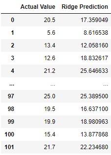
Let’s see how we can use this technique with Sci-Kit Learn. As we mentioned, when we use a different values for alpha, we get different results. In this example we use value 10 for this hyperparameter:
ridge_reg = make_pipeline(StandardScaler(), Ridge(alpha=10, solver="cholesky"))
ridge_reg.fit(X_train, y_train)
ridge_reg_predictions = ridge_reg.predict(X_test)

pd.DataFrame({
    'Actual Value': y_test,
    'Ridge Prediction': ridge_reg_predictions,
})
We can see that results are a bit better for higher values. As mentioned this can be used with stochastic gradient descent regression like this:
sgd_ridge_reg = make_pipeline(StandardScaler(), SGDRegressor(penalty="l2"))
sgd_ridge_reg.fit(X_train, y_train)
sgd_ridge_reg_predictions = sgd_ridge_reg.predict(X_test)

pd.DataFrame({
    'Actual Value': y_test,
    'SGD Ridge Prediction': sgd_ridge_reg_predictions,
})
Let’s see how this compare with linear regression when we plot the results:

As we can see the results are close to each other.
Lasso Regression
Least Absolute Shrinkage and Selection Operator Regression or Lasso regularization technique that follows similar principles as Ridge. It adds regularization term to the cost function, but it uses L1 Norm. The regularization parameter is αΣ |θi| meaning that if we use MSE as a cost function the new cost function looks like this:

From the equation, you can see that penalizes only high coefficients. The really interesting thing about this regression is its ability to completely eliminate the coefficients of the least important features. Meaning it does some kind of feature selection, by choosing features that are essential to predictions. Eventually, it produces a sparse model, which increases model explainability. The downside is that Lasso regression function is not differentiable at θi = 0 (for i = 1, 2, ⋯, n). However, we can still use Gradient Descent with a subgradient vector.
Using Sci-Kit Learn
We use Lasso from Sci-Kit Learn to perform this operation on the Boston Housing dataset:
lasso_reg = make_pipeline(StandardScaler(), Lasso(alpha=1))
lasso_reg.fit(X_train, y_train)
lasso_reg_predictions = lasso_reg.predict(X_test)

pd.DataFrame({
    'Actual Value': y_test,
    'Lasso Prediction': lasso_reg_predictions,
})
We can see that results are different and interesting. When we use it with Stochastic Gradient Descent, we get this:
sgd_lasso_reg = make_pipeline(StandardScaler(), SGDRegressor(penalty="l1"))
sgd_lasso_reg.fit(X_train, y_train)
sgd_lasso_reg_predictions = sgd_lasso_reg.predict(X_test)

pd.DataFrame({
    'Actual Value': y_test,
    'SGD Lasso Prediction': sgd_lasso_reg_predictions,
})
Finally, let’s plot out the compared results:

Elastic Net
However, what we should do if neither of these options produces the aimed result. Well, then you can use both of them. Kinda. Elastic Net is a regularization technique that combines Lasso and Ridge. Both regularization terms are added to the cost function, with one additional hyperparameter r. This hyperparameter controls the Lasso-to-Ridge ratio. In a nutshell, if r = 0 Elastic Net performs Ridge regression and if r = 1 it performs Lasso regression. This means that the cost function of Elastic Net can be represented as (taken that MSE is the cost function we want to use):

Using Sci-Kit Learn
Here is how we use it with Sci-Kit Learn:
elastic_net_reg = make_pipeline(StandardScaler(), ElasticNet(alpha=0.1, l1_ratio=0.5))
elastic_net_reg.fit(X_train, y_train)
elastic_net_reg_predictions = elastic_net_reg.predict(X_test)

pd.DataFrame({
    'Actual Value': y_test,
    'ElasticNet Prediction': elastic_net_reg_predictions,
})
And plot it out:

In general, it is good to know that it is always good to have at least a bit of regularization. This means that we should avoid using pure Linear Regression. Ridge is a way to go if we want good performance and it is a great default. If we suspect that there might be features that are useless in our dataset, we can go with Elastic Net or Lasso.
Early Stopping
Another regularization technique is Early Stopping. This is a non-mathematical technique that Geoffrey Hinton called a “beautiful free lunch“. The main trick of this technique is to stop training as soon as the validation error reaches a minimum. Essentially, the model is saved after each epoch and assessing the performance of the model on the validation set. When we use Gradient Descent cost should decrease after each epoch and with it, validation error as well. Theoretically, at least.

However, if the model starts overfitting validation error can start increasing which is an indication that the performance of the model decreases. There are two ways that this technique can be implemented. The first one is to stop the training right after validation error starts increasing. The other way is training the model for a fixed number of epochs, saving models at each epoch (checkpoint) and then picking the one with the best results. The second approach is typical for training neural networks. Some of the algorithms in the Sci-Kit Learn Library have hyperparameter which you can use to set up this process easily. Let’s see where we will land with Boston Housing Dataset:
sgd_reg = SGDRegressor(penalty="elasticnet", early_stopping = True, alpha=11)
X_train = StandardScaler().fit_transform(X_train)

sgd_reg.fit(X_train, y_train)
sgd_reg_predictions = sgd_reg.predict(X_test)

pd.DataFrame({
    'Actual Value': y_test,
    'SGD with early stopping': sgd_reg_predictions,
})
We got some really weird results like this, just look at the plot:

Ugh! As it turned out, we need additional experiments with this approach and further hyperparameter tuning, or it might not be a good approach to our problem at all. Anyhow, now you know the meaning of this process and how to use it with Sci-Kit Learn.
Conclusion
In this article we had a chance to explore how we can utilize unsupervised learning for clustering problems. We observed three algorithms K-Means CLustering, Hierarchical Clustering and DBSCAN. We applied them to PalmerPenguins dataset and saw some really interesting results. Also, we had a chance to see how powerfull unsupervised learning can be.
Thank you for reading!

Nikola M. Zivkovic
CAIO at Rubik's Code
Nikola M. Zivkovic a CAIO at Rubik’s Code and the author of book “Deep Learning for Programmers“. He is loves knowledge sharing, and he is experienced speaker. You can find him speaking at meetups, conferences and as a guest lecturer at the University of Novi Sad.
Rubik’s Code is a boutique data science and software service company with more than 10 years of experience in Machine Learning, Artificial Intelligence & Software development. Check out the services we provide.


Trackbacks/Pingbacks