So far in our journey through the Machine Learning universe, we covered several big topics. We investigated some regression algorithms, classification algorithms and algorithms that can be used for both types of problems (SVM, Decision Trees and Random Forest). Apart from that, we dipped our toes in unsupervised learning, saw how we can use this type of learning for clustering and learned about several clustering techniques.
We also talked about how to quantify machine learning model performance and how to improve it with regularization. In all these articles, we used Python for “from the scratch” implementations and libraries like TensorFlow, Pytorch and SciKit Learn. The word optimization popped out more than once in these articles, so in this article, we focus on optimization techniques which are an important part of the machine learning process.
This bundle of e-books is specially crafted for beginners.
Everything from Python basics to the deployment of Machine Learning algorithms to production in one place.
Become a Machine Learning Superhero TODAY!
In general, every machine learning algorithm is composed of three integral parts:
- A loss function.
- Optimization criteria based on the loss function, like a cost function.
- Optimization technique – this process leverages training data to find a solution for optimization criteria (cost function).
As you were able to see in previous articles, some algorithms were created intuitively and didn’t have optimization criteria in mind. In fact, mathematical explanations of why and how these algorithms work were done later. Some of these algorithms are Decision Trees and kNN. Other algorithms, which were developed later had this thing in mind beforehand. SVM is one example.

During the training, we change the parameters of our machine learning model to try and minimize the loss function. However, the question of how do you change those parameters arises. Also, by how much should we change them during training and when. To answer all these questions we use optimizers. They put all different parts of the machine learning algorithm together.
So far we mentioned Gradient Decent as an optimization technique, but we haven’t explored it in more detail. In this article, we focus on that and we cover the grandfather of all optimization techniques and its variation. Note that these techniques are not machine learning algorithms. They are solvers of minimization problems in which the function to minimize has a gradient in most points of its domain.
In this article we cover:
- Dataset & Prerequsites
- Why do we use Optimizers?
- Gradient Descent Intuition
- Gradient Descent Deeper Dive
- Gradient Descent Implementation with Python
- Batch Gradient Descent Intuition
- Batch Gradient Descent Implementation with Python
- Stohastic Gradient Descent Intuition
- Stohastic Gradient Descent Implementation with Python
- Stohastic Gradient Descent Implementation with Python
1. Dataset & Prerequisites
Data that we use in this article is the famous Boston Housing Dataset. This dataset is composed 14 features and contains information collected by the U.S Census Service concerning housing in the area of Boston Mass. It is a small dataset with only 506 samples.

For the purpose of this article, make sure that you have installed the following Python libraries:
- NumPy – Follow this guide if you need help with installation.
- SciKit Learn – Follow this guide if you need help with installation.
- Pandas – Follow this guide if you need help with installation.
Once installed make sure that you have imported all the necessary modules that are used in this tutorial.
import pandas as pd
import numpy as np
import matplotlib.pyplot as plt

from sklearn.model_selection import train_test_split
from sklearn.metrics import mean_squared_error
from sklearn.preprocessing import StandardScaler
from sklearn.linear_model import SGDRegressor
Apart from that, it would be good to be at least familiar with the basics of linear algebra, calculus and probability.
2. Why do we use Optimizers?
Note that we also use simple Linear Regression in all examples. Due to the fact that we explore optimization techniques, we picked the easiest machine learning algorithm. You can see more details about Linear regression here. As a quick reminder the formula for linear regression goes like this:

where w and b are parameters of the machine learning algorithm. The entire point of the training process is to set the correct values to the w and b, so we get the desired output from the machine learning model. This means that we are trying to make the value of our error vector as small as possible, i.e. to find a global minimum of the cost function.
One way of solving this problem is to use calculus. We could compute derivatives and then use them to find places where is an extrema of the cost function. However, the cost function is not a function of one or a few variables; it is a function of all parameters of a machine learning algorithm, so these calculations will quickly grow into a monster. That is why we use these optimizers.
3. Gradient Descent Intuition
This technique is the most popular optimization techniques. It is also a basis for other techniques as well. There is one useful analogy that describes this process quite well. Imagine that you had a ball inside a rounded valley like in the picture below. If you let the ball roll, it will go from one side of the valley to the other, until it goes still at the bottom.
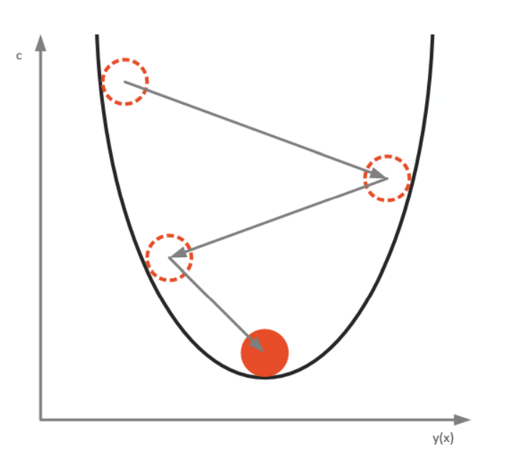
Essentially, we can look at this behavior like the ball is optimizing its position from left to right, and eventually, it stops at the bottom, i.e. the lowest point of the bowl. The bottom, in this case, is the minimum of our cost function. This is what the gradient descent algorithm is doing. It starts from one position in which by calculating derivatives and second derivatives of cost function it gets the information about where “the ball” should roll. Every time we calculate derivatives we get information about the slope of the side of the function (i.e. bowl) at its current position.

When the slope is negative (downward from left to right), the ball should move to the right, otherwise, it should move to the left. Be aware that the ball is just an analogy, and we are not trying to develop an accurate simulation of the laws of physics. We are trying to get to the minimum of the function using this alternative method since we already realized that using calculus is not optimal.

In a nutshell, the training process of Linear Regression with Gradient Descent can be described like this:
- Put the training set in the machine algorithm and get the output for each sample in it,
- The output is compared with the desired output and error is calculated using a cost function,
- Based on the error value and used cost function, a decision on how the w and b should be changed is made in order to minimize the error value,
- The process is repeated until the error is minimal.
4. Gradient Descent Deeper Dive
Let’s formalize this in more mathematical terms. We don’t know what the optimal values for w and b are in the Linear Regression formula:

Let’s formalize this in more mathematical terms. We don’t know what the optimal values for w and b are in the Linear Regression formula:

where N is the number of samples in the dataset, yi is the real output value and xi is the input vector (where each feature is represented with a separate coordinate). The first step in the Gradient Descent would be to define partial derivates for each parameter. For w, we use chain rule and get the result:

and for b we get:

Once we know how to calculate partial derivatives for all parameters in the machine learning model (in this case w and b) for the defined cost function (in this case MSE), then we can initialize values for tose parameters (w and b). The initialization process is a completely different topic outside of the scope of this tutorial. So, in this article, we will initialize those values to 0. Then we start iteration through the training set examples and update w and b, by utilizing partial derivatives after each sample:

where alpha is the learning rate hyperparameter. This hyperparameter controls how “strong” an update is. When we go through all examples in the training set we call that an epoch. In general, we train our machine learning algorithms for multiple epochs.
5. Gradient Descent Implementation with Python
Ok, that is enough theory, let’s implement this with Python. The complete implementation is done within MyGradientDescent class:
class MyGradientDescent():
    def __init__(self, learning_rate):
        self.learning_rate = learning_rate
        self.w = 0
        self.b = 0

    def fit(self, X, y, epochs = 100):
        N = len(X)
        history = []

        for e in range(epochs):
            for i in range(N):
                Xi = X[i, :]
                yi = y[i, :]

                f = yi - (self.w * Xi + self.b)

                self.w -= self.learning_rate * (-2 * Xi.dot(f.T).sum() / N)
                self.b -= self.learning_rate * (-2 * f.sum() / N)

            loss = mean_squared_error(y, (self.w * X + self.b))

            if e % 100 == 0:
                print(f"Epoch: {e}, Loss: {loss})")

            history.append(loss)

        return history

    def predict(self, X):
        return self.w * X + self.b
It is a pretty simple class. Note that name of this class is maybe not completely accurate. In essence, we created an algorithm that uses Linear regression with Gradient Descent. This is important to say. Here the algorithm is still Linear Regression, but the method that helped us we learn w and b is Gradient Descent. We could switch to any other learning algorithm.
In the constructor of the class, we initialize the value of w and b to zero. Also, we initialize the learning rate hyperparameter. There are two public methods:
- fit – This is the method that performs the training process. Note that it returns history, where we record loss during training. This is done for future visualizations. Apart from that for updating w and b we used formulas defined above.
- predict – Method that predicts value.
Note that for the loss we use MSE and in the code, we use Sci-Kit learn function to calculate it. Let’s utilize this class on the data:
model = MyGradientDescent(learning_rate = 0.01)
history = model.fit(X_train, y_train, 1000)

predictions = model.predict(X_test)
Epoch: 0, Loss: 1.0129236386713547)
Epoch: 100, Loss: 0.4836365268936342)
Epoch: 200, Loss: 0.4717052013642623)
Epoch: 300, Loss: 0.4714309129514397)
Epoch: 400, Loss: 0.4714244612434121)
Epoch: 500, Loss: 0.47142429776534295)
Epoch: 600, Loss: 0.4714242918194498)
Epoch: 700, Loss: 0.4714242913200272)
Epoch: 800, Loss: 0.47142429124768254)
Epoch: 900, Loss: 0.47142429123592733)We can see how our algorithm is diverging because the loss is slowly going down. Once it is done we can plot the history and see how the loss function decreased during training process:

Another thing we can do is to plot the final model:

Also, we can compare real values with predictions (keep in mind that data is scaled):

The biggest problem of the Gradient Descent is that it can converge towards a local minimum and not to a global one. In our case that is not a problem, since MSE is a convex function that has just one minimum – a global one. The other problem is that for big datasets this approach can take some time.
6. Batch Gradient Descent Intuition
However, in practice, it would be inefficient to calculate the partial gradient of the cost function for each small change in the w or b, for each sample. You could see that it is not the fastest approach. That is why simple optimization is done, ie. partial derivative is calculated for a complete set of parameters in one go. For MSE, that is done using the formula:

where θ is the set of all machine learning parameters. In our case, θ0 is b while other θ values come from w. This optimized version is of gradient descent is called batch gradient descent, due to the fact that partial gradient descent is calculated for complete input X (i.e. batch) at each gradient step. This means that w and b can be updated using the formulas:

7. Batch Gradient Descent Implementation with Python
The implementation of this algorithm is very similar to the implementation of “vanilla” Gradient Descent. We do so in the class MyBatchGradientDescent:
class MyBatchGradientDescent():
    def __init__(self, learning_rate):
        self.learning_rate = learning_rate
        self.w = 0
        self.b = 0

    def fit(self, X, y, epochs = 100):
        N = len(X)
        history = []

        for e in range(epochs):
            f = y - (self.w * X + self.b)

            self.w -= self.learning_rate * (-2 * X.dot(f.T).sum() / N)
            self.b -= self.learning_rate * (-2 * f.sum() / N)

            loss = mean_squared_error(y, (self.w * X + self.b))

            if e % 100 == 0:
                print(f"Epoch: {e}, Loss: {loss})")

            history.append(loss)

        return history

    def predict(self, X):
        return self.w * X + self.b
The only difference is the way we update w and b. When we fit our data in this algorithm, here is what we get:
model = MyBatchGradientDescent(learning_rate = 0.01)
history = model.fit(X_train, y_train, 1000)

predictions = model.predict(X_test)
Epoch: 0, Loss: 1.0196646159305187)
Epoch: 100, Loss: 0.6771864255196849)
Epoch: 200, Loss: 0.6660374373514026)
Epoch: 300, Loss: 0.6655591433109558)
Epoch: 400, Loss: 0.6655383319190815)
Epoch: 500, Loss: 0.6655374258171037)
Epoch: 600, Loss: 0.6655373863654891)
Epoch: 700, Loss: 0.6655373846477667)
Epoch: 800, Loss: 0.6655373845729767)
Epoch: 900, Loss: 0.6655373845697203)Even though this approach is faster, we got some different results with it, loss is a bit higher than the one when we used simple gradient descent. Perhaps we should train it more. This difference can also be seen with the model that this approach created:
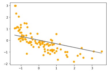
And in the results that it outputs:

8. Stohastic Gradient Descent Intuition
Stochastic gradient descent (SGD) is an updated version of the Batch Gradient Descent algorithm that speeds up the computation by approximating the gradient using smaller subsets of the training data. These subsets are called mini-batches or just batches.
Sometimes in literature, you will find that Stochastic Gradient Descent is a version on Gradient Dataset that picks one random sample from the input dataset and that Mini-Batch Gradient Descent takes a subset of samples from the input dataset. However, those formal lines are a bit blurred in the day to day work.
If someone says that they use stochastic gradient descent, it is high chances that they are referring to the one that uses the mini-batches. After all one sample is just a subset with one element. In this article, we are using this context – that Stochastic Gradient Descent uses mini-batches which are the subset of the input dataset.
Since this algorithm works with considerably less data than Batch Gradient Descent it is faster. Also, this means that this algorithm can be used on big datasets. However, due to its random nature, this process is much less regularized. The loss will not linearly go to it’s minimum, but it will bounce up and down until it stabilizes and diverges. Let’s see how the implementation of this algorithm looks like in Python.
9. Stohastic Gradient Descent Implementation with Python
Ok, the only thing that we need to improve from the previous implementation is to give the user of our class the ability to define the size of the batch. Here is how we do it in the class MySGD:
class MySGD():
    def __init__(self, learning_rate):
        self.learning_rate = learning_rate
        self.w = 0
        self.b = 0

    def _get_batch(self, X, y, batch_size):
        indexes = np.random.randint(len(X), size=batch_size)
        return X[indexes,:], y[indexes,:]

    def fit(self, X, y, batch_size = 32, epochs = 100):
        N = len(X)
        history = []

        for e in range(epochs):
            indexes = np.random.randint(N, size=batch_size)
            X_batch, y_batch = self._get_batch(X, y, batch_size)

            f = y_batch - (self.w * X_batch + self.b)

            self.w -= self.learning_rate * (-2 * X_batch.dot(f.T).sum() / N)
            self.b -= self.learning_rate * (-2 * f.sum() / N)

            loss = mean_squared_error(y_batch, (self.w * X_batch + self.b))

            if e % 100 == 0:
                print(f"Epoch: {e}, Loss: {loss})")

            history.append(loss)

        return history

    def predict(self, X):
        return self.w * X + self.b
You can see one additional private function _get_batch. This method retrieves a random subset of input and output data for the training. It is the only difference from MyBatchGradientDescent class. The fit method is modified to utilize this method and generate X_batch and y_batch, which are later on used in the training. Ok, let’s try this on our dataset:
model = MySGD(learning_rate = 0.01)
history = model.fit(X_train, y_train, batch_size = 64, epochs = 1000)

predictions = model.predict(X_test)
Epoch: 0, Loss: 0.6988926574320093)
Epoch: 100, Loss: 0.9368940114609687)
Epoch: 200, Loss: 0.38274490789600646)
Epoch: 300, Loss: 0.4015009827201944)
Epoch: 400, Loss: 0.6096862052672033)
Epoch: 500, Loss: 0.4814101552252322)
Epoch: 600, Loss: 0.3249126077150954)
Epoch: 700, Loss: 0.6309038218016978)
Epoch: 800, Loss: 0.6394188763053792)
Epoch: 900, Loss: 0.6521754136964174)From the output, we can see that loss is going up and down, which we expected, but notice how overall loss is going down. We can observe that when we plot the history:
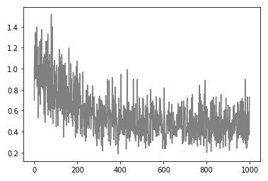
Even though this seems a bit odd at first, observe what happens when we plot the predictions and compare it with the results we got from Batch Gradient Descent:
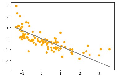
We got a better approximation of the data! And with that we got more accurate predictions:

10. Stohastic Gradient Descent Implementation with SciKit Learn
As it usually goes, everything we write from scratch already exists in the Sci-Kit Learn library, which makes our lives a lot easier. Let’s use SGDRegressor for our problem:
sgd_model = SGDRegressor(max_iter=10000, alpha=0.1)
sgd_model.fit(X_train, y_train)

sgd_predictions = sgd_model.predict(X_test)
Quite straightforward, nothing more than we seen so far. Note that the alpha parameter is the learning rate and max_iter is the maximal number of epochs. When we plot the result, we get the more or less same thing as our implementation:

The same goes with the table of results:

Conclusion
In this article we got a chance to see how Gradient Descent, the most commonly used optimization technique, works. It is the optimization technique from which all started. We had a chance to implement it from scratch using Python and see how we can utilize it with Sci-Kit learn. In the next article, we will cover some other more advanced optimization techniques which are based on a notion of momentum.
Thank you for reading!

Nikola M. Zivkovic
Author at Rubik's Code
Nikola M. Zivkovic a CAIO at Rubik’s Code and the author of books: Ultimate Guide to Machine Learning and Deep Learning for Programmers. He loves knowledge sharing, and he is an experienced speaker. You can find him speaking at meetups, conferences, and as a guest lecturer at the University of Novi Sad.


Very interesting article. Thank you for posting this. Pls can you show how to solve this problem using the gradient descent method: https://projecteuler.net/problem=607