We know that we used logo from Transformers in the featured image, so if you are a toy/movies/cartoon fan, sorry to disappoint you. We won’t cover any of those topics in this blog post. However, if you are data science and deep learning fan, you are in the right place. In this article, we explore the interesting architecture of Transformers. They are a special type of sequence-to-sequence models used for language modeling, machine translation, image captioning and text generation.

Generally speaking, sequence-to-sequence models are a type of models that receives a sequence of input data and provides another sequence of data as an output. This is completely different from Standard Feed Forward Neural Networks and Convolutional Neural Networks, which are accepting a fixed-size vector as input and produce a fixed-sized vector as an output. For example if you want to translate sentence “You are awesome.” from English to Serbian, sequence-to-sequence model will receive word by word as an input and generate output “Ti si super”.

This is more aligned with the way humans think as well. Meaning, we are not throwing everything away and start every thought from the scratch. We use context and the information we received beforehand. As you are reading this your understanding of every word is based on your understanding of previous words.

Of course, behind the cartons is where the spooky stuff is happening. These models are essentially created of two main components: Encoder and Decoder. These are both essentially Recurrent Neural Networks (more on them in the next chapter). The Encoder is the component which receives each part of the input sequence. Then it encodes it (duh!) into a vector, which is called – context. This context carries information about the whole sequence and it is sent over to the Decoder. This component of sequence-to-sequence model is able to understand the context and resolve it into meaningful output.

In this site, we already covered two predominant types of sequence-to-sequence models: Recurrent Neural Networks (RNN) and Long-Short Term Memory Networks (LSTM). LSTMs are essentially built on top of the idea of RNNs. However, these type of networks didn’t fully satisfied the needs. Thus the Transformers were introduced back in 2017. in the paper with an awesome title “Attention is all you need“. Let’s refresh our memory a bit and remind ourselves what are the good and the bad things about the RNNs and the LSTMs.

Recurrent Neural Networks

The structure of Recurrent Neural Networks is similar to the structure of Standard Feed Neural Networks, but with one major twist. They are propagating output of the network back to the input. Wait, what? Yes, we are using the output of the network in time moment T to calculate the output of the network in moment T + 1. Take a look at this oversimplified representation of RNN:

This means that output will be sent back to the input and then used when next input comes along, in next time step. Basically, “state” of the network is forward propagated through time. RNNs are somewhat time traveling neural networks. If unroll this structure, so to say we can represent the same thing like this:

To sum it up, RNNs have “memory” in which they store information about information in the process thus far. So, if we use sentence “You are awesome.” as an input to RNN, it will first process the word “You”. Then it will process word “are” but using output of the word “You” as well. Either way, you get the picture, we are using some sort of a process to combine an output of previous time step and input in current time step to calculate output in current time step. To find out more about this type of neural networks check this article.

One of the perks of using RNNs is that we can connect previous information to the present task and based on that make certain predictions. For example, we can try to predict what will be the next word in the certain sentence based on the previous word from the sentence. RNNs are great for this kind of tasks. However, we rarely need to look only one step back to perform a certain task .

Take that example of text prediction in language modeling. Sometimes we can predict next word in the text based on the previous one, but more often we need more information than just the previous word. We need context, we need more words from the sentence. Apart from that, exploding/vanishing gradient problem is even more probable in these networks, since we carry information through time (backpropagation through time). That is where LSTMs come into picture.

Long-Short Term Memory Networks (LSTMs)

In order to address problems that RNNs have, Hochreiter & Schmidhuber came up with the concept of Long Short-Term Memory Networks back in 1997. The structure is similar to the structure of standard RNN, meaning they feed output information back to the input, but these networks don’t struggle with problems that standard RNNs do. In their architecture, they have implemented a mechanism for remembering long dependencies.

They do so by instead of a single layer, they have four and they have more operations regarding those four levels. Example of single LSTM unit’s structure can be seen in the image below:

Here is the legend for elements from this graph above:

As you can see in the image we have four network layers. One layer is using the tahn activation function and two layers are using the sigmoid activation function. Apart form that, we are having some pointwise operations and regular operations on the vectors, like concatenation. The important thing to notice however is the data stream marked with the letter C. This represents memory that is holding information outside of the rest of the network and is known as the cell state.  

If we over simplify the way that LSTMs work, we can say that this process is done through several steps. Firstly, LSTMs forget unnecessary information from the cell state. Then they add new information into it and finally they calculate the output. Now, it is a bit more complicated than that, so if you want to find out how it functions in details, check this article.

While this architecture improves RNNs a lot, it is still far from ideal. When sentences get too long LSTMs don’t do too well. Mathematically speaking, the probability of keeping the context from a word that is far away from the current word being processed decreases exponentially with the distance. Another problem is that this sequential process cannot be done in parallel, so training of these networks takes quite a lot of time.

Attention

All problems of RNNs and LSTMs can be traced back to the context vector. In an essence, this vector is a bottleneck of the whole system. One solution was proposed by Minh-Thang Luong back in 2015. and even in its title it contained intriguing word and concept – Attention. What does this word means from the machine learning perspective? Basically, attention allows the model to focus on the relevant and important parts of the input sequence as needed. Sequence-to-sequence models with attention differ from the vanilla ones in several ways.

Thus far we saw how Encoder passes only the last hidden state as a context to the Decoder. When we use attention, the Encoder sends all hidden states to the Decoder. Apart from that, the Decoder does some extra processing before producing the output. This is done because now every hidden state that the Encoder has sent is associated with certain part of the input sequence. In the example “You are awesome.”, first hidden state in the context would be related to the word “You”, second hidden state would be related to the word “are”, and so on. The Decoder has more information now, so it can make use of it.

Firstly, the Decoder calculates the weight of each hidden state that is sent by the Encoder. This is done using the Decoder’s hidden state (i.e. output of the previous time step). Then it softmaxes these weights. This way the Decoder gives advantage to the hidden states with high weight values. Finally, it multiplies each hidden state with the softmaxed weight and sums them up. This way new context vector with attention to important parts is created.

This context is then used as an input to the Decoder’s feed forward neural network, which provides an output item of the sequence. This output is used as hidden state of the Decoder and it is used for the calculation of the weights in the next time step.

Self – Attention

Ok, the attention is one cool concept that the Decoder use. How about the Encoder? Anything special about it? The “Attention is all you need“ paper we mentioned previously introduces one more interesting concept that Transformers utilize called self-attention. The goal of this concept is to associate two items from the input sequence. In this example, we used Tensor2Tensor notebook, which is pretty cool for visualization of self-attention. Let’s observe the sentence we want to translate:

The animal didn't cross the street because it was too tired. 

To be more precise, let’s observe the word “it” in this sentence. To us, humans, it is pretty clear that this word refers to the word “animal” from the first part of the sentence. However, a machines don’t know this. As the Encoder processes each item from the input sequence, concept of self – attention gives it the ability to look for clues in other items form the input sequence, in order to better encode it. Just like RNN uses hidden state to get the information about previous item from the sequence, the Encoder uses self-attention to extract understanding of currently processed item from other inputs in the sequence.

How does it work? Well, this process can be divided into 6 steps:

1. For each item of the input sequence three vectors are calculated: Query – q, Key – k and Value – v. They are calculated by applying three matrices we create during the training process.
2. Calculating score for each item in the input sequence by doing dot product of the Query vector with the Key vector of other items in the sequence. In our example from previous chapter, if we are calculating self-attention for the word “You”, we create score for each word in the sentence against this word. Meaning we calculate dot products of q(You) and k(You), q(You) and k(are) and q(You) and k(awesome).
3. Divide scores with 8 (other value can be used as well, but this one is default).
4. Apply the softmax function. That way scores are normalized, positive and add up to 1.
5. Multiply Value vector with the softmaxed score from the step 4.
6. Sum up all the results into single vector and create the output of the self-attention.

Of course, in order to speed up this process calculation is done on matrices not on vectors, bu the process is the same. Output of this self-attention layer is than passed to the feed forward neural network. This is just a high overview of this concept, so we suggest you explore this topic further and check out “Attention is all you need“ paper.

Transformers

Transformers essentially uses all the aforementioned concepts and fits them together. They give fantastic results in the machine translation tasks. How do they do it? From the high level perspective they don’t look much different from the standard sequence-to-sequence model we explored so far. Except from the cool logo, of course 🙂

However, when we look under the Transformer’s hood (pun intended), we can see something different. We can see bunch of encoders and decoders stacked one on top of each other. In the initial paper that proposed this architecture, it is used 6 encoders and 6 decoders. Other number can be used as well.

Each encoder is composed of two parts: Self-Attention Layer and Feed Forward Neural Network, while each decoder have three parts: Self-Attention Layer, Decoder Attention Layer and Feed Forward Neural Network. That looks something like this:

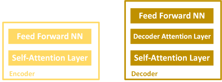
The first Encoder receives a list of input vectors. When we are working with words this is usually an output of some kind of Embedding layer. It process them by using self-attention layer and then feed-forward neural network. Afterwards it sends that output to the next Encoder. The final Encoder sends this information to the Decoders, which perform similar process.

Conclusion

In this article we got a chance to get familiar with several concepts. First we reminded ourselves about use cases for sequence-to-sequence models and some of the architectures we were able to explore thus far. We saw what RNNs and LSTMs bring to the table and what are their pitfalls. Apart from that, we saw how the concepts of Attention and Self-Attention are implemented in deep learning and how it is utilized in Transformers architecture.

Thank you for reading!

---

Read more posts from the author at Rubik’s Code.

---