
In the previous article, we got a chance to get familiar with the architecture of Transformer. Not just that, but we explored all architectures that came before it and what problems did they have, like Recurrent Neural Networks and Long Short Term Memory Networks. We also had a chance to see how sequence-to-sequence models function in general, and how Transformers architecture build on top of that using concepts like Attention. In this and next couple of articles we will be able to see how one can implement one of these monumental architectures using Python and TensorFlow. There are a lot of separate components that need to be implemented and understood and that is why this implementation is separated into several articles.

To be more precise, in this mini-series of articles we will implement one Transformer solution that will be able to translate Russian into English. Since the whole concept of Transformer architecture revolves around the idea of Attention, this first article will be focused more on that part of the architecture. Essentially, Transformer is able to handle variable-sized input using stacks of these self-attention layers. That is why we will focus on that part of implementation. Apart from that, since we are creating a model that works with sequences of words, this article will present some concepts that will help us prepare data in a manner that it will be best processed with the model in the end. In order to understand Transformer architecture from the higher level check this article.
Throughout this implementation we will heavily rely on the amazing “Attention is all you need” paper. In this paper the architecture of each encoder and decoder are presented like this:

We will focus on the marked sections in this first article.
Prerequisites

In order to run the code from this article, you have to have Python 3 installed on your local machine. In this example, to be more specific, we are using Python 3.7. The implementation itself is done using TensorFlow 2.0. The complete guide on how to install and use Tensorflow 2.0 can be found here. Another thing that you need to install is TensorFlow Datasets (TFDS) package. You can do so by running the command:
pip install tensorflow-datasets
This module contains a large database of data sets that can be used for training purposes. We will use one of these data sets for our model. Here is the list of modules that needs to be imported for the complete Transformer implementation:
| import tensorflow_datasets as tfds | |
| import tensorflow as tf | |
| from tensorflow.keras.layers import Layer, Dense, LayerNormalization, Embedding, Dropout | |
| from tensorflow.keras.models import Sequential, Model | |
| from tensorflow.keras.optimizers.schedules import LearningRateSchedule | |
| from tensorflow.keras.optimizers import Adam | |
| from tensorflow.keras.losses import SparseCategoricalCrossentropy | |
| from tensorflow.keras.metrics import Mean, SparseCategoricalAccuracy | |
| from tqdm import tqdm | |
| import numpy as np | |
| import matplotlib.pyplot as plt |
Make sure that you have them all installed.
Data Handling

As we already mentioned, the goal of this model is to translate Russian into English. This means that we want to map knowledge about the relationships between words in Russian language into English language. This type of learning is often referred to as deep translation. Generally speaking it is any operation where we try to map prior knowledge from one domain into a different domain. In this particular case we use that with language. “How do machine knows so much about Russian language?” one might ask.
Lucky for us, TFDS contains data set that has word embeddings used for neural machine translations. This data set is provided by the TED Talks Open Translation Project and more information on it can be found here. In this example we use one particular “sub-data set” – ted_hrlr_translate/ru_to_en . These specific embeddings contain separate information about semantically similar words in English and in Russian language separately. We will talk more about concept of Embedding into next chapter. The goal of the Transformer is to map knowledge of one domain into another one. This corpus of words contains around 20000 training examples, 5000 validation examples, and 5000 test examples. The information about this data set says:
| tfds.core.DatasetInfo( | |
| name='ted_hrlr_translate', | |
| version=0.0.1, | |
| description='Data sets derived from TED talk transcripts for comparing similar language pairs | |
| where one is high resource and the other is low resource. | |
| ', | |
| urls=['https://github.com/neulab/word-embeddings-for-nmt'%5D, | |
| features=Translation({ | |
| 'en': Text(shape=(), dtype=tf.string), | |
| 'ru': Text(shape=(), dtype=tf.string), | |
| }), | |
| total_num_examples=218387, | |
| splits={ | |
| 'test': 5476, | |
| 'train': 208106, | |
| 'validation': 4805, | |
| }, | |
| supervised_keys=('ru', 'en'), | |
| citation="""@inproceedings{Ye2018WordEmbeddings, | |
| author = {Ye, Qi and Devendra, Sachan and Matthieu, Felix and Sarguna, Padmanabhan and Graham, Neubig}, | |
| title = {When and Why are pre-trained word embeddings useful for Neural Machine Translation}, | |
| booktitle = {HLT-NAACL}, | |
| year = {2018}, | |
| }""", | |
| redistribution_info=, | |
| ) |
One sample from this data set, looks something like this before processing:

Since text data is typically variable length, in order to prepare it for processing we need to pad it. Also, we need to break up each sequence, i.e sentence, into words. This process is called tokenization. To sum it up, we need to brake every sentence into words. Integer value needs to be assigned to each word. Additionally, we will not use sequences that have more than 30 words. To make this process easier we create class called DataHandler. Here is the code:
| class DataHandler(object): | |
| def __init__(self, word_max_length = 30, batch_size = 64, buffer_size = 20000): | |
| train_data, test_data = self._load_data() | |
| self.tokenizer_ru = tfds.features.text.SubwordTextEncoder.build_from_corpus((ru.numpy() for ru, en in train_data), target_vocab_size=2**13) | |
| self.tokenizer_en = tfds.features.text.SubwordTextEncoder.build_from_corpus((en.numpy() for ru, en in train_data), target_vocab_size=2**13) | |
| self.train_data = self._prepare_training_data(train_data, word_max_length, batch_size, buffer_size) | |
| self.test_data = self._prepare_testing_data(test_data, word_max_length, batch_size) | |
| def _load_data(self): | |
| data, info = tfds.load('ted_hrlr_translate/ru_to_en', with_info=True, as_supervised=True) | |
| return data['train'], data['validation'] | |
| def _prepare_training_data(self, data, word_max_length, batch_size, buffer_size): | |
| data = data.map(self._encode_tf_wrapper) | |
| data.filter(lambda x, y: tf.logical_and(tf.size(x) <= word_max_length, tf.size(y) <= word_max_length)) | |
| data = data.cache() | |
| data = data.shuffle(buffer_size).padded_batch(batch_size, padded_shapes=([-1], [-1])) | |
| data = data.prefetch(tf.data.experimental.AUTOTUNE) | |
| return data | |
| def _prepare_testing_data(self, data, word_max_length, batch_size): | |
| data = data.map(self._encode_tf_wrapper) | |
| data = data.filter(lambda x, y: tf.logical_and(tf.size(x) <= word_max_length, tf.size(y) <= word_max_length)).padded_batch(batch_size, padded_shapes=([-1], [-1])) | |
| def _encode(self, english, russian): | |
| russian = [self.tokenizer_ru.vocab_size] + self.tokenizer_ru.encode(russian.numpy()) + [self.tokenizer_ru.vocab_size+1] | |
| english = [self.tokenizer_en.vocab_size] + self.tokenizer_en.encode(english.numpy()) + [self.tokenizer_en.vocab_size+1] | |
| return russian, english | |
| def _encode_tf_wrapper(self, pt, en): | |
| return tf.py_function(self._encode, [pt, en], [tf.int64, tf.int64]) |
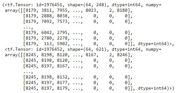
In the constructor of this class we load the data. Apart from that, we create two SubwordTextEncoder objects – tokenizers. One is for English language and the other for Russian. The goal of each tokenizer is to encode the string by breaking it into sub-words if the word is not already in its dictionary. In function _encode and its TensorFlow wrapper _encode_tf_wrapper, we add start and end token. The whole process of preparing the data is handled in _prepare_training_data method, where we tokenize, enconde and pad the sequences. We filter the ones which are too long here as well. One sample from this dataset, looks something like this after processing:
Embedding and Positional Encoding

We already mentioned Embedding, so let’s see what it is all about. Essentially, this process transforms text into a numerical representation, a vector, based on it’s semantic meaning. This means that words will be transferred into some sort of vector representation (or embedding) in n-dimensional latent space. In this space, vectors that are close to each other belong to the words that have similar semantic meaning. For example, “sound” and “headphones” have close embeddings, while “sound” and “chair” do not. In the same manner, words from different languages and same meaning have close embeddings. This means that, in this example, words “data” and “данные” will have close embeddings. These embeddings are, as you were able to see, already given in the data set.
As we can see, embeddings give us information about semantically similar words. However, semantic meaning of the word can depend on the position of that word in a sentence and on relationship with other words in that same sentence. That is why we need additional information about relative position of every word in a sequence. That information is transferred using positional encoding vector. This process is proposed in the “Attention is all you need” paper. You can find more about how relative position can be found using current position of the word in this paper. To sum it up, positional encoding vector is added to the already existing embeddings. This vector is calculated using the formulas:


where pos is possition, i is the dimension and d is the dimension of embedding. In order to handle creation of this vector we create class PositionalEncoding:
| class PositionalEncoding(object): | |
| def __init__(self, position, d): | |
| angle_rads = self._get_angles(np.arange(position)[:, np.newaxis], np.arange(d)[np.newaxis, :], d) | |
| sines = np.sin(angle_rads[:, 0::2]) | |
| cosines = np.cos(angle_rads[:, 1::2]) | |
| self._encoding = np.concatenate([sines, cosines], axis=-1) | |
| self._encoding = self._encoding[np.newaxis, …] | |
| def _get_angles(self, position, i, d): | |
| angle_rates = 1 / np.power(10000, (2 * (i//2)) / np.float32(d)) | |
| return position * angle_rates | |
| def get_positional_encoding(self): | |
| return tf.cast(self._encoding, dtype=tf.float32) |
Essentially, we just implemented formulas from above into this class. Here is how it can be used:
| positional_encoding = PositionalEncoding(50, 512) | |
| positional_encoding_values = positional_encoding.get_positional_encoding() | |
| print("Positional Encoding Example:") | |
| print("———–") | |
| print(positional_encoding_values) | |
| print("———–") |
The output looks something like this:

Soon we will see how this concept is used as a part of attention layers.
Masks

Remember how we said that we have to do the padding, so our sequences have the same length? That is necessary for the processing, however, we need a mechanism to tell to our model to ignore that padding because it doesn’t carry any information. Cool thing is that we already used SubwordTextEncoder for tokenization. This class inherits abstract TextEncoder class that handles this situation and use value 0 for padding. This means that encoding will never have value 0, while decoding drops 0 in input. Apart from that, when we look for size of the vocabulary these values are included and we get proper padded dimensions.
Another problem is that we somehow need to indicate to the model that it needs to process only words before the current word. This means that to predict the fourth word, only the first, second and the third word are used, but not the fifth. Both of those problems, padding and future words, are solved using masks. For this purpose, we create the class MaskHandler:
| class MaskHandler(object): | |
| def padding_mask(self, sequence): | |
| sequence = tf.cast(tf.math.equal(sequence, 0), tf.float32) | |
| return sequence[:, tf.newaxis, tf.newaxis, :] | |
| def look_ahead_mask(self, size): | |
| mask = 1 – tf.linalg.band_part(tf.ones((size, size)), -1, 0) | |
| return mask |
Function padding_mask handles the first problem, while function look_ahead_mask handles the second problem. Here is the example of usage of this class:
| maskHandler = MaskHandler() | |
| x = tf.constant([[1, 2, 0, 0, 6], [1, 1, 1, 0, 0], [0, 0, 0, 6, 9]]) | |
| mask = maskHandler.padding_mask(x) | |
| print("Padding Mask Example:") | |
| print("———–") | |
| print(mask) | |
| print("———–") | |
| x = tf.random.uniform((1, 3)) | |
| mask = maskHandler.look_ahead_mask(x.shape[1]) | |
| print("Look Ahead Mask Example:") | |
| print("———–") | |
| print(mask) | |
| print("———–") |
In the output we can see the example of both type of masks:

Attention Layers

Attention is a concept that allows Transformer to focus on a specific parts of the sequence, i.e. sentence. It can be described as mapping function, because in its essence it maps a query and a set of key-value pairs to an output. Query, keys, values, and output are all vectors. The output is calculated as a weighted sum of the values, where the weight assigned to each value is computed by a compatibility function of the query with the corresponding key. The whole process can be divided into 6 steps:
- For each item of the input sequence three vectors are calculated: Query – q, Key – k and Value – v. They are calculated by applying three matrices we create during the training process.
- Calculating score for each item in the input sequence by doing dot product of the Query vector with the Key vector of other items in the sequence. In our example from previous chapter, if we are calculating self-attention for the word “You”, we create score for each word in the sentence against this word. Meaning we calculate dot products of q(You) and k(You), q(You) and k(are) and q(You) and k(awesome).
- Divide scores with 8 (other value can be used as well, but this one is default).
- Apply the softmax function. That way scores are normalized, positive and add up to 1.
- Multiply Value vector with the softmaxed score from the step 4.
- Sum up all the results into single vector and create the output of the self-attention.
In this article, we will examine two types of attention layers: Scaled dot Product Attention and Multi-Head Attention.
Scaled Dot-Product Attention
The attention used in Transformer is best known as Scaled Dot-Product Attention. This layer can be presented like this:

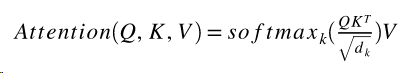
As in other attention layers, the input of this layer contains of queries and keys (with dimension dk), and values (with dimension dv). We calculate the dot products of the query with all keys. Then we divide each by square root of dk and apply a softmax function. Mathematically this layer can be described with the formula:
This layer is implemented within the class ScaledDotProductAttentionLayer:
| class ScaledDotProductAttentionLayer(): | |
| def calculate_output_weights(self, q, k, v, mask): | |
| qk = tf.matmul(q, k, transpose_b=True) | |
| dk = tf.cast(tf.shape(k)[-1], tf.float32) | |
| scaled_attention = qk / tf.math.sqrt(dk) | |
| if mask is not None: | |
| scaled_attention_logits += (mask * -1e9) | |
| weights = tf.nn.softmax(scaled_attention, axis=-1) | |
| output = tf.matmul(weights, v) | |
| return output, weights |
Multi-Head Attention Layer
Building on top of previous layer, it has been noticed that when we linearly project the queries, keys and values n-times with different projections, we get better results. This means that instead of one single attention “head” (i.e. Scaled Dot-Product Layer), Q, K, and V are split into multiple “heads”. This way the model can attend to information at different positions from different representational spaces. That is how idea of Multi-Head Attention Layer is born. Here is how it looks like:

Essentially, it performs four steps. First this layer gets three inputs – Q, K, V, and splits them using linear layer into three branches or “heads”. Then scaled dot-product attention is applied on each “head”. Results are then concatenated and passed to the final linear layer. Mathematically Multi-Head Attention Layer can be presented with the formula:

This layer is implemented within the class MultiHeadAttentionLayer:
| class MultiHeadAttentionLayer(Layer): | |
| def __init__(self, num_neurons, num_heads): | |
| super(MultiHeadAttentionLayer, self).__init__() | |
| self.num_heads = num_heads | |
| self.num_neurons = num_neurons | |
| self.depth = num_neurons // self.num_heads | |
| self.attention_layer = ScaledDotProductAttentionLayer() | |
| self.q_layer = Dense(num_neurons) | |
| self.k_layer = Dense(num_neurons) | |
| self.v_layer = Dense(num_neurons) | |
| self.linear_layer = Dense(num_neurons) | |
| def split(self, x, batch_size): | |
| x = tf.reshape(x, (batch_size, -1, self.num_heads, self.depth)) | |
| return tf.transpose(x, perm=[0, 2, 1, 3]) | |
| def call(self, v, k, q, mask): | |
| batch_size = tf.shape(q)[0] | |
| # Run through linear layers | |
| q = self.q_layer(q) | |
| k = self.k_layer(k) | |
| v = self.v_layer(v) | |
| # Split the heads | |
| q = self.split(q, batch_size) | |
| k = self.split(k, batch_size) | |
| v = self.split(v, batch_size) | |
| # Run through attention | |
| attention_output, weights = self.attention_layer.calculate_output_weights(q, k, v, mask) | |
| # Prepare for the rest of processing | |
| output = tf.transpose(attention_output, perm=[0, 2, 1, 3]) | |
| concat_attention = tf.reshape(output, (batch_size, -1, self.num_neurons)) | |
| # Run through final linear layer | |
| output = self.linear_layer(concat_attention) | |
| return output, weights |
Conclusion
In this article, we started implementation of Transformer Architecture. We had a chance to see how to prepare data from TFDS and how to create first few steps in the Transformer architecture, like Positional Encoding, masking and attention. In the next article, we will implement Encoder and Decoder Layers completely.
Thank you for reading!
Read more posts from the author at Rubik’s Code.


What did you use for drawing thos diagrams, such as multi headed attention.
Hey there,
I used MS Visio.
Thanks for reading 🙂