The code that accompanies this article can be found here.
So far in our journey through the Machine Learning universe, we covered several big topics. We investigated some regression algorithms, classification algorithms and algorithms that can be used for both types of problems (SVM, Decision Trees and Random Forest). Apart from that, we dipped our toes in unsupervised learning, saw how we can use this type of learning for clustering and learned about several clustering techniques.
We also talked about how to quantify machine learning model performance and how to improve it with regularization. In all these articles, we used Python for “from the scratch” implementations and libraries like TensorFlow, Pytorch and SciKit Learn. In the previous article, we covered the topic of Gradient Descent, the grandfather of all optimization techniques. Following down that path, we explore momentum-based optimizers and the optimizers that scale the learning rate.
Are you afraid that AI might take your job? Make sure you are the one who is building it.
STAY RELEVANT IN THE RISING AI INDUSTRY! 🖖
Gradient Descent keeps track only of the gradient from the previous step, which can make it slow. If the gradient is small, meaning that the slope is not that big, it will take it some time until the minimum is reached. Essentially, this is the problem that optimizers that we explore are trying to solve. These optimizers are more often used with neural networks than with regular machine learning algorithms. However, in order to simplify explanations, we use linear regression for all explanations. As in the previous article, it is important to note that these techniques are not machine learning algorithms. They are solvers of minimization problems in which the function to minimize has a gradient in most points of its domain.

As a quick reminder the formula for linear regression goes like this:

where w and b are parameters of the machine learning algorithm. The entire point of the training process is to set the correct values to the w and b, so we get the desired output from the machine learning model. This means that we are trying to make the value of our error vector as small as possible, i.e. to find a global minimum of the cost function.
Dataset & Prerequisites
Data that we use in this article is the famous Boston Housing Dataset. This dataset is composed 14 features and contains information collected by the U.S Census Service concerning housing in the area of Boston Mass. It is a small dataset with only 506 samples.

For the purpose of this article, make sure that you have installed the following Python libraries:
- NumPy – Follow this guide if you need help with installation.
- SciKit Learn – Follow this guide if you need help with installation.
- Pandas – Follow this guide if you need help with installation.
Once installed make sure that you have imported all the necessary modules that are used in this tutorial.
import pandas as pd
import numpy as np
import matplotlib.pyplot as plt

from sklearn.model_selection import train_test_split
from sklearn.metrics import mean_squared_error
from sklearn.preprocessing import StandardScaler
Apart from that, it would be good to be at least familiar with the basics of linear algebra, calculus and probability.
Preparing the Data
The preparation of this data is simple and follows the examples from previous articles. Here is how we do it. First, we load data using Pandas and drop all samples that have empty values:
data = pd.read_csv('./data/boston_housing.csv')
data = data.dropna()
Then create instance of the StandardScaler, because we want to put our data in same scale. Also, we isolate input and output data. For inputs we use only ‘lstat‘ feature and for output we use ‘medv‘ feature. On these features we use scaler:
scaler = StandardScaler()

X = data['lstat'].values
X = X.reshape(-1, 1)
X = scaler.fit_transform(X)

y = data['medv'].values
y = y.reshape(-1, 1)
y = scaler.fit_transform(y)
Finally, we split data into training and testing datasets:
X_train, X_test, y_train, y_test = train_test_split(X, y, test_size=0.2, random_state=33)When we plot the data here is what it looks like:

Momentum Optimizer
In order to improve this, a new version of optimizers was born – Momentum Optimizers. Essentially, this idea was born back in 1974 by Boris T. Polyak and they are focused on helping models converge as fast as possible. The idea comes from observing a ball rolling down a gentle slope. It will start off slowly, but it will gain momentum. So, the core of the idea is to focus on movement in the correct direction. This is done by reducing the variance in every other insignificant direction and thus accelerating gradient descent.

Moment Optimization introduces the momentum vector. This vector is used to “store” changes in previous gradients. This vector helps accelerate stochastic gradient descent in the relevant direction and dampens oscillations. At each gradient step, the local gradient is added to the momentum vector. Then parameters are updated just by subtracting the momentum vector from the current parameter values. Since the whole idea kinda comes from physics, a new hyperparameter β is introduced – momentum. It simulates the friction mechanism and regulates the momentum value so it doesn’t explode. Typically this value is set to 0.9. To sum it up, momentum optimization is performed in two steps:
1. Calculating momentum vector at each iteration using the formula:

where m is momentum vector, β is momentum, α is learning rate, θ is the set of machine learning parameters and ∇MSE is the partial derivative of the cost function (Mean Squared Error in this case).
2. Update the parameters by subtracting the momentum vector.

Python Implementation
We implement this algorithm within MyMomentumOptimizer class:
class MyMomentumOptimizer():
    def __init__(self, learning_rate, momentum = 0.9):
        self.learning_rate = learning_rate
        self.momentum = momentum

        self.w = 0
        self.b = 0

        self.momentum_vector_w = 0
        self.momentum_vector_b = 0

    def _get_batch(self, X, y, batch_size):
        indexes = np.random.randint(len(X), size=batch_size)
        return X[indexes,:], y[indexes,:]

    def _get_momentum_vector(self, X_batch, y_batch):
        f = y_batch - (self.w * X_batch + self.b)

        self.momentum_vector_w = self.momentum * self.momentum_vector_w + \
                                 self.learning_rate * (-2 * X_batch.dot(f.T).sum() / len(X_batch))
        self.momentum_vector_b = self.momentum * self.momentum_vector_b + \
                                 self.learning_rate * (-2 * f.sum() / len(X_batch))

    def fit(self, X, y, batch_size = 32, epochs = 100):
        history = []

        for e in range(epochs):

            indexes = np.random.randint(len(X), size=batch_size)
            X_batch, y_batch = self._get_batch(X, y, batch_size)

            self._get_momentum_vector(X_batch, y_batch)

            self.w -= self.momentum_vector_w
            self.b -= self.momentum_vector_b

            loss = mean_squared_error(y_batch, (self.w * X_batch + self.b))

            if e % 100 == 0:
                print(f"Epoch: {e}, Loss: {loss})")

            history.append(loss)

        return history

    def predict(self, X):
        return self.w * X + self.b
Ugh, that is a lot of code, let’s chuck it up and explain piece by piece. In the constructor of this class, we initialize the necessary attributes and set hyperparameter values. Learning rate and momentum are set, and algorithm parameters w and b are initialized to 0. The same goes for momentum vectors. Note that we could put all the parameters of the algorithm (w and b) within one array, but we wanted everything to be as clear as possible. The code can, of course, be improved.
def __init__(self, learning_rate, momentum = 0.9):
	self.learning_rate = learning_rate
	self.momentum = momentum

	self.w = 0
	self.b = 0

	self.momentum_vector_w = 0
	self.momentum_vector_b = 0
Two private methods _get_batch and _get_momentum_vector are very important. Method _get_batch is used to pick batch from the input and output datasets. Method _get_momentum_vector does the dirty work we defined in the momentum algorithm. Here the gradient for each parameter is calculated (you can find formulas for this in the previous article) and used to update the momentum vector for each parameter.
def _get_batch(self, X, y, batch_size):
	indexes = np.random.randint(len(X), size=batch_size)
	return X[indexes,:], y[indexes,:]

def _get_momentum_vector(self, X_batch, y_batch):
	f = y_batch - (self.w * X_batch + self.b)

	self.momentum_vector_w = self.momentum * self.momentum_vector_w + \
				 self.learning_rate * (-2 * X_batch.dot(f.T).sum() / len(X_batch))
	self.momentum_vector_b = self.momentum * self.momentum_vector_b + \
				 self.learning_rate * (-2 * f.sum() / len(X_batch))
Finally, in the fit method, the actual training is performed. For each epoch, this algorithm first fetches the batch and calculates momentum vectors for each parameter. In the end, w and b are updated using these vectors. Apart from that, we calculate the loss, print it out, and store it in history. This is done just so we can follow what is happening during the training process. The method predict just predicts values for the input.
def fit(self, X, y, batch_size = 32, epochs = 100):
	history = []

	for e in range(epochs):

		indexes = np.random.randint(len(X), size=batch_size)
		X_batch, y_batch = self._get_batch(X, y, batch_size)

		self._get_velocity(X_batch, y_batch)

		self.w -= self.velocity_w
		self.b -= self.velocity_b

		loss = mean_squared_error(y_batch, (self.w * X_batch + self.b))

		if e % 100 == 0:
			print(f"Epoch: {e}, Loss: {loss})")

		history.append(loss)

	return history

def predict(self, X):
	return self.w * X + self.b
Now when we understand what is happening in this class, let’s run this on loaded data:
model = MyMomentumOptimizer(learning_rate = 0.0001)
history = model.fit(X_train, y_train, batch_size = 128, epochs = 1000)

predictions = model.predict(X_test)
Epoch: 0, Loss: 1.023970350020749)
Epoch: 100, Loss: 0.8915269977932345)
Epoch: 200, Loss: 0.6160710091923012)
Epoch: 300, Loss: 0.7748865586040383)
Epoch: 400, Loss: 0.7624729068019713)
Epoch: 500, Loss: 0.7386694964887148)
Epoch: 600, Loss: 0.4590078364639633)
Epoch: 700, Loss: 0.45645337845296935)
Epoch: 800, Loss: 0.548081143220535)
Epoch: 900, Loss: 0.5855308679385105)We can note that this algorithm goes to the global minimum quite quickly, which is what we wanted. Also, note that it is almost as momentum optimizer goes fast “ahead” and then backs up. If we plot the loss history we get something like this:
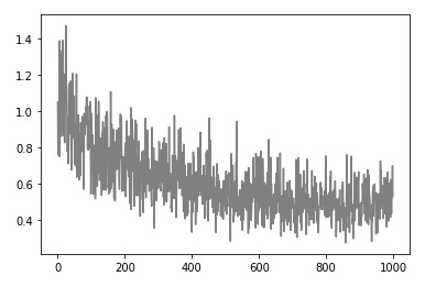
And if we plot the model it looks something like this:

Seems quite cool that we were able to get really good results with this approach, taken into consideration that we are using Linear Regression as our chosen algorithm.
Nesterov Accelerated Gradient
Yurii Nesterov noticed, back in 1983, that it is possible to improve momentum based optimization and make it go to the global minimum even faster. Let’s use our ball analogy once again. Imagine having a smarter ball, that will detect when it rolled over the minimum and slow down even more. That is an analogy that we can take when talking about the difference between classical momentum optimization and Nesterov Accelerated Gradient.

The trick is just to measure the gradient of the cost function “in the future” and adapt according to that. What does this mean? Well since we know the momentum vector, we can calculate the gradient of the cost function slightly ahead in the direction of the momentum vector. This will give us gives us an approximation of the next position of the parameters, ie. a rough idea about future values of our parameters. Here is how we update the momentum vector then:

The meaning of all symbols is the same as in the previous formula. Essentially, the only difference is that we calculate the partial gradient of cost function not in regards with parameters θ, but in regards to θ + βm. We update the parameters in the same way as for the classical momentum:

This small change of perspective results in a faster algorithm than simple momentum. This is especially useful when working with neural networks. Let’s find out how that looks like in code.
Python Implementation
The implementation of this algorithm looks almost the same to the MyMomentumOptimizer class. Take a look at MyNestrovAcceleratedGradient class that contains that implementation:
class MyNestrovAcceleratedGradient():
    def __init__(self, learning_rate, momentum = 0.9):
        self.learning_rate = learning_rate
        self.momentum = momentum

        self.w = 0
        self.b = 0

        self.momentum_vector_w = 0
        self.momentum_vector_b = 0

    def _get_batch(self, X, y, batch_size):
        indexes = np.random.randint(len(X), size=batch_size)
        return X[indexes,:], y[indexes,:]

    def _get_momentum_vector(self, X_batch, y_batch):
        f = y_batch - ((self.w + self.momentum * self.momentum_vector_w) * X_batch + \
	    (self.momentum * self.momentum_vector_b))

        self.momentum_vector_w = self.momentum * self.momentum_vector_w + \
                                 self.learning_rate * (-2 * X_batch.dot(f.T).sum() / len(X_batch))

        self.momentum_vector_b = self.momentum * self.momentum_vector_b + \
                                 self.learning_rate * (-2 * f.sum() / len(X_batch))

    def fit(self, X, y, batch_size = 32, epochs = 100):
        history = []
        momentum_vector = np.zeros_like(1)

        for e in range(epochs):

            indexes = np.random.randint(len(X), size=batch_size)
            X_batch, y_batch = self._get_batch(X, y, batch_size)

            self._get_momentum_vector(X_batch, y_batch)

            self.w -= self.momentum_vector_w
            self.b -= self.momentum_vector_b

            loss = mean_squared_error(y_batch, (self.w * X_batch + self.b))

            if e % 100 == 0:
                print(f"Epoch: {e}, Loss: {loss})")

            history.append(loss)

        return history

    def predict(self, X):
        return self.w * X + self.b
Ok, this is almost the same. The only difference can be seen in the function _get_momentum_vector, which is in charge of calculating the momentum vector when we calculate the loss function. For the classical momentum we use:
f = y_batch - (self.w * X_batch + self.b)However, instead of that, for Nesterov Accelerated Gradient we use:
f = y_batch - ((self.w + self.momentum * self.velocity_w) * X_batch + \
    (self.momentum * self.velocity_b))
Apart from that, the rest of implementation is the same. The API is the same so we can use it just like the other algorithms from this series:
model = MyNestrovAcceleratedGradient(learning_rate = 0.0001)
history = model.fit(X_train, y_train, batch_size = 128, epochs = 1000)

predictions = model.predict(X_test)
Epoch: 0, Loss: 1.0428307224941038)
Epoch: 100, Loss: 0.7708240506795851)
Epoch: 200, Loss: 0.9109097502153849)
Epoch: 300, Loss: 0.576534368060239)
Epoch: 400, Loss: 0.3422810954841916)
Epoch: 500, Loss: 0.556215628177696)
Epoch: 600, Loss: 0.35335516341041334)
Epoch: 700, Loss: 0.39640988193508453)
Epoch: 800, Loss: 0.5852076539641191)
Epoch: 900, Loss: 0.5284027213990843)Notice that loss is a bit smaller. Here is what the history looks like:

Finally, we can plot out the model:

There is one more way we can improve optimization. Momentum-based optimizers focused on adding some value to the complete formula, but the other approach is to modify the learning rate, i.e to control the scaling of the gradient. One such algorithm is AdaGrad.
AdaGrad
AdaGrad and similar algorithms focus on adaptively scaling the learning rate for each dimension. If we go back to our ball analogy (I would like to say for the last time but I can not promise that :)), this algorithm quickly detects where is the global minimum early on and pushes the ball in its direction. It is almost like putting some magnet in at the global minimum.
How does it work? Well, it is performed in two steps. First, we calculate scale vector – s:

this vector accumulates the squares of the partial derivative of the cost function with regards to the parameter. The vector s is then used to scale the learning rate:

where ε is the so-called smoothing term hyperparameter, which is set to some small value like 10^-10. Essentially, this means that this algorithm adapts the learning rate to the parameters, performing smaller updates for parameters associated with frequently occurring features, and larger updates for parameters associated with infrequent features. This is why this optimizer is frequently used in combination with neural networks and sparse data.
Python Implementation
The implementation of this algorithm can be found in MyAdaGrad class:
class MyAdaGrad():
    def __init__(self, learning_rate, epsilon = 10 ** -10):
        self.learning_rate = learning_rate
        self.epsilon = epsilon

        self.w = 0
        self.b = 0

        self.scale_w = 0
        self.scale_b = 0

    def _get_batch(self, X, y, batch_size):
        indexes = np.random.randint(len(X), size=batch_size)
        return X[indexes,:], y[indexes,:]

    def _get_scale(self, X_batch, y_batch):
        f = y_batch - (self.w * X_batch + self.b)

        gradient_w = (-2 * X_batch.dot(f.T).sum() / len(X_batch))
        gradient_b = (-2 * f.sum() / len(X_batch))

        self.scale_w += np.multiply(gradient_w, gradient_w)
        self.scale_b += np.multiply(gradient_b, gradient_b)

    def fit(self, X, y, batch_size = 32, epochs = 100):
        history = []
        momentum_vector = np.zeros_like(1)

        for e in range(epochs):

            indexes = np.random.randint(len(X), size=batch_size)
            X_batch, y_batch = self._get_batch(X, y, batch_size)

            self._get_scale(X_batch, y_batch)

            f = y_batch - (self.w * X_batch + self.b)

            divider_w = np.sqrt(self.scale_w + self.epsilon)
            divider_b = np.sqrt(self.scale_b + self.epsilon)

            gradient_w = (-2 * X_batch.dot(f.T).sum() / len(X_batch))
            gradient_b = (-2 * f.sum() / len(X_batch))

            self.w -= self.learning_rate * gradient_w / divider_w
            self.b -= self.learning_rate * gradient_b / divider_b

            loss = mean_squared_error(y_batch, (self.w * X_batch + self.b))

            if e % 100 == 0:
                print(f"Epoch: {e}, Loss: {loss})")

            history.append(loss)

        return history

    def predict(self, X):
        return self.w * X + self.b
Let’s break it down! In the constructor we initialize all the necessary parameters (w and b), however, we initialize s values for those parameters as well. Apart from that note that learning rate is not the only hyperparameter, but we have ε value which we set to some small value close to zero.
def __init__(self, learning_rate, epsilon = 10 ** -10):
        self.learning_rate = learning_rate
        self.epsilon = epsilon

        self.w = 0
        self.b = 0

        self.scale_w = 0
        self.scale_b = 0
While the _get_batch method is the same as for previous algorithms, we have a new _get_scale method which calculates s vector for each parameter. That is done by multiplying gradient of the cost function with itself:
def _get_batch(self, X, y, batch_size):
        indexes = np.random.randint(len(X), size=batch_size)
        return X[indexes,:], y[indexes,:]

def _get_scale(self, X_batch, y_batch):
        f = y_batch - (self.w * X_batch + self.b)

        gradient_w = (-2 * X_batch.dot(f.T).sum() / len(X_batch))
        gradient_b = (-2 * f.sum() / len(X_batch))

        self.scale_w += np.multiply(gradient_w, gradient_w)
        self.scale_b += np.multiply(gradient_b, gradient_b)
Finally, in the fit method, we first get the batch and calculate the s vector. Then we calculate “the divider”, ie. the factor using which we divide the learning rate. After that parameters w and b are updated:
def fit(self, X, y, batch_size = 32, epochs = 100):
        history = []
        momentum_vector = np.zeros_like(1)

        for e in range(epochs):

            indexes = np.random.randint(len(X), size=batch_size)
            X_batch, y_batch = self._get_batch(X, y, batch_size)

            self._get_scale(X_batch, y_batch)

            f = y_batch - (self.w * X_batch + self.b)

            divider_w = np.sqrt(self.scale_w + self.epsilon)
            divider_b = np.sqrt(self.scale_b + self.epsilon)

            gradient_w = (-2 * X_batch.dot(f.T).sum() / len(X_batch))
            gradient_b = (-2 * f.sum() / len(X_batch))

            self.w -= self.learning_rate * gradient_w / divider_w
            self.b -= self.learning_rate * gradient_b / divider_b

            loss = mean_squared_error(y_batch, (self.w * X_batch + self.b))

            if e % 100 == 0:
                print(f"Epoch: {e}, Loss: {loss})")

            history.append(loss)

        return history

def predict(self, X):
        return self.w * X + self.b
When we use this implementation with the data here is what we get:
model = MyAdaGrad(learning_rate = 0.1)
history = model.fit(X_train, y_train, batch_size = 128, epochs = 1000)

predictions = model.predict(X_test)
Epoch: 0, Loss: 0.7979041986313373)
Epoch: 100, Loss: 0.5538556882638777)
Epoch: 200, Loss: 0.47179562048530943)
Epoch: 300, Loss: 0.6090468657219893)
Epoch: 400, Loss: 0.29050695867780074)
Epoch: 500, Loss: 0.3170492333098174)
Epoch: 600, Loss: 0.5305147131291987)
Epoch: 700, Loss: 0.45605887968605396)
Epoch: 800, Loss: 0.4405627012256315)
Epoch: 900, Loss: 0.6149532862507887)If we plot out the loss, we will notice that it goes down way faster than with momentum-based algorithms.
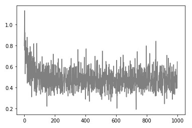
The model looks pretty much the same:

RMSProp
RMSProp builds on AdaGrad ideas. It is another adaptive learning rate method proposed by Geoff Hinton. Since Adagrad tends to be too aggressive and never converging to the global optimum, RMSProp proposes a solution for that. In essence, this algorithm restricts the accumulation of gradients by using a decay hyperparameter.

So instead of adding complete square gradient to the s vector every iteration, it does it like this:

where betta is the decay hyperparameter. Hinton proposed a value of 0.9 for β and 0.001 for the learning rate. The parameter update is done in the same way as for AdaGrad:

Python Implementation
As you can imagine implementation of this algorithm is similar to MyAdaGrad class. Here is what code of MyRMSProp class looks like:
class MyRMSProp():
    def __init__(self, learning_rate, decay_rate = 0.9, epsilon = 10 ** -10):
        self.learning_rate = learning_rate
        self.epsilon = epsilon
        self.decay_rate = decay_rate

        self.w = 0
        self.b = 0

        self.scale_w = 0
        self.scale_b = 0

    def _get_batch(self, X, y, batch_size):
        indexes = np.random.randint(len(X), size=batch_size)
        return X[indexes,:], y[indexes,:]

    def _get_scale(self, X_batch, y_batch):
        f = y_batch - (self.w * X_batch + self.b)

        gradient_w = (-2 * X_batch.dot(f.T).sum() / len(X_batch))
        gradient_b = (-2 * f.sum() / len(X_batch))

        self.scale_w = self.decay_rate * self.scale_w + \
     		       (1 - self.decay_rate) * np.multiply(gradient_w, gradient_w)
        self.scale_b = self.decay_rate * self.scale_b + \
		       (1 - self.decay_rate) * np.multiply(gradient_b, gradient_b)

    def fit(self, X, y, batch_size = 32, epochs = 100):
        history = []
        momentum_vector = np.zeros_like(1)

        for e in range(epochs):

            indexes = np.random.randint(len(X), size=batch_size)
            X_batch, y_batch = self._get_batch(X, y, batch_size)

            self._get_scale(X_batch, y_batch)

            f = y_batch - (self.w * X_batch + self.b)

            divider_w = np.sqrt(self.scale_w + self.epsilon)
            divider_b = np.sqrt(self.scale_b + self.epsilon)

            gradient_w = (-2 * X_batch.dot(f.T).sum() / len(X_batch))
            gradient_b = (-2 * f.sum() / len(X_batch))

            self.w -= self.learning_rate * gradient_w / divider_w
            self.b -= self.learning_rate * gradient_b / divider_b

            loss = mean_squared_error(y_batch, (self.w * X_batch + self.b))

            if e % 100 == 0:
                print(f"Epoch: {e}, Loss: {loss})")

            history.append(loss)

        return history

    def predict(self, X):
        return self.w * X + self.b
The difference we can notice here is the decay hyperparameter. It is initialized through the constructor and used for scale vector calculation. For AdaGrad we calculated scale vector like this:
self.scale_w += np.multiply(gradient_w, gradient_w)
self.scale_b += np.multiply(gradient_b, gradient_b)
In this algorithm we do so like this:
self.scale_w = self.decay_rate * self.scale_w + \
	       (1 - self.decay_rate) * np.multiply(gradient_w, gradient_w)
self.scale_b = self.decay_rate * self.scale_b + \
 	       (1 - self.decay_rate) * np.multiply(gradient_b, gradient_b)
Here is what we get when we use RMSProp with Boston Housing data:
model = MyRMSProp(learning_rate = 0.01)
history = model.fit(X_train, y_train, batch_size = 128, epochs = 2000)

predictions = model.predict(X_test)
Epoch: 0, Loss: 1.0067302568004783)
Epoch: 100, Loss: 0.5548727653729529)
Epoch: 200, Loss: 0.4650584261906152)
Epoch: 300, Loss: 0.5603081231881148)
Epoch: 400, Loss: 0.6147792885402231)
Epoch: 500, Loss: 0.5129763511682113)
Epoch: 600, Loss: 0.591699424069597)
Epoch: 700, Loss: 0.5413949069489516)
Epoch: 800, Loss: 0.5215547915706193)
Epoch: 900, Loss: 0.48122559852723423)
Epoch: 1000, Loss: 0.497310753056444)
Epoch: 1100, Loss: 0.38403636517387396)
Epoch: 1200, Loss: 0.3829499207052695)
Epoch: 1300, Loss: 0.4287416366915751)
Epoch: 1400, Loss: 0.48688055753943527)
Epoch: 1500, Loss: 0.41232863743069914)
Epoch: 1600, Loss: 0.3436122983294806)
Epoch: 1700, Loss: 0.4730678956784552)
Epoch: 1800, Loss: 0.4586441383688593)
Epoch: 1900, Loss: 0.4893198589718893)The loss definitely goes down slower, but it converges. Take a look at the loss history:

Here is what we get when we plot the model:

Adam
It is pretty standard that several techniques are combined in the world of the data science. That is how the Adam optimizer was born – by combining good things from momentum based optimizers mixed with good things from adaptive learning rate optimizers. By the way, Adam stands for adaptive moment estimation, but the altorithm is deffinitly more intuitive than its name. It combines ideas from momentum based optimization and RMSProp, meaning it keeps both exponentially decaying average of past gradients and squared gradients.

Here is how this algorithm is defined:

Where βm is momentum decay, βs is scale decay and t is the epoch (starting from 1). The βm hyperparameter is usually set to 0.9 and βs to value close to one, like 0.95 or 9.99. The second and fourth step of this process might be a bit confusing, so let’s reflect on them for a bit. Because momentum and scale vectors are initialized to 0 at the beginning of this algorithm, they can be biased to 0 at the beginning of training. These steps are making sure that doesn’t happen.
At the moment, this is one of the most popular optimizers. Let’s implement it.
Python Implementation
The MyAdam class contains the implementation of the Adam algorithm. It is a combination of MyMomentumOptimizer class and MyRMSProp class with a twist. Take a look:
class MyAdam():
    def __init__(self, learning_rate, momentum_decay = 0.9, scaling_decay = 0.95, epsilon = 10 ** -8):
        self.learning_rate = learning_rate
        self.epsilon = epsilon
        self.momentum_decay = momentum_decay
        self.scaling_decay = scaling_decay
        self.w = 0
        self.b = 0
        self.scale_w = 0
        self.scale_b = 0
        self.momentum_vector_w = 0
        self.momentum_vector_b = 0

    def _get_batch(self, X, y, batch_size):
        indexes = np.random.randint(len(X), size=batch_size)
        return X[indexes,:], y[indexes,:]

    def _get_gradients(self, X_batch, y_batch):
        f = y_batch - (self.w * X_batch + self.b)

        gradient_w = (-2 * X_batch.dot(f.T).sum() / len(X_batch))
        gradient_b = (-2 * f.sum() / len(X_batch))

        return gradient_w, gradient_b

    def _get_momentum_vector(self, X_batch, y_batch, gradient_w, gradient_b, epoch):
        self.momentum_vector_w = self.momentum_decay * self.momentum_vector_w + (1 - self.momentum_decay) * gradient_w
        self.momentum_vector_b = self.momentum_decay * self.momentum_vector_b + (1 - self.momentum_decay) * gradient_b

        self.momentum_vector_w = self.momentum_vector_w / (1 - self.momentum_decay**epoch)
        self.momentum_vector_b = self.momentum_vector_b / (1 - self.momentum_decay**epoch)

    def _get_scale(self, X_batch, y_batch, gradient_w, gradient_b, epoch):
        self.scale_w = self.scaling_decay * self.scale_w + (1 - self.scaling_decay) * np.multiply(gradient_w, gradient_w)
        self.scale_b = self.scaling_decay * self.scale_b + (1 - self.scaling_decay) * np.multiply(gradient_b, gradient_b)

        self.scale_w = self.scale_w / (1 - self.scaling_decay**epoch)
        self.scale_b = self.scale_b / (1 - self.scaling_decay**epoch)

    def fit(self, X, y, batch_size = 32, epochs = 100):
        history = []
        momentum_vector = np.zeros_like(1)

        for e in range(epochs):

            indexes = np.random.randint(len(X), size=batch_size)
            X_batch, y_batch = self._get_batch(X, y, batch_size)

            gradient_w, gradient_b = self._get_gradients(X_batch, y_batch)

            self._get_scale(X_batch, y_batch, gradient_w, gradient_b, e + 1)
            self._get_momentum_vector(X_batch, y_batch,gradient_w, gradient_b, e + 1)

            divider_w = np.sqrt(self.scale_w + self.epsilon)
            divider_b = np.sqrt(self.scale_b + self.epsilon)

            self.w -= self.learning_rate * self.momentum_vector_w * gradient_w / divider_w
            self.b -= self.learning_rate * self.momentum_vector_b * gradient_b / divider_b

            loss = mean_squared_error(y_batch, (self.w * X_batch + self.b))

            if e % 100 == 0:
                print(f"Epoch: {e}, Loss: {loss})")

            history.append(loss)

        return history

    def predict(self, X):
        return self.w * X + self.b
There are some new moments there. The constructor is huge now because it has to handle additional hyperparameters and initialize both scale and momentum vectors. We also extracted the _get_gradients method, so we can quickly get gradients for both parameters. The _get_scale and _get_velocity methods are similar to the previous implementations, but they are using βm and βs hyperparameters according to the Adam algorithm definition. The fit method follows these steps:
- Get batch
- Calculate gradients
- Calculate momentum vector
- Calculate scale vector
- Update parameters
When we apply it to our data:
model = MyAdam(learning_rate = 0.001)
history = model.fit(X_train, y_train, batch_size = 32, epochs = 2000)

predictions = model.predict(X_test)
Epoch: 0, Loss: 1.6016804863141227)
Epoch: 100, Loss: 1.0708601616598528)
Epoch: 200, Loss: 0.8396258429842761)
Epoch: 300, Loss: 0.9498729862073851)
Epoch: 400, Loss: 1.422709838725747)
Epoch: 500, Loss: 0.951641965926126)
Epoch: 600, Loss: 0.5114273687678832)
Epoch: 700, Loss: 0.9474342613915748)
Epoch: 800, Loss: 0.18370682522157994)
Epoch: 900, Loss: 0.551880807891246)
Epoch: 1000, Loss: 0.8319923072193909)
Epoch: 1100, Loss: 0.47982450339753563)
Epoch: 1200, Loss: 0.6607618450191821)
Epoch: 1300, Loss: 0.5550136613614162)
Epoch: 1400, Loss: 0.3261014705384321)
Epoch: 1500, Loss: 0.8596159351953009)
Epoch: 1600, Loss: 0.4764163861345504)
Epoch: 1700, Loss: 0.4233869971005261)
Epoch: 1800, Loss: 0.8254322188333079)
Epoch: 1900, Loss: 0.5054093932889874)Here is what history of loss looks like:

Model still looks good as well:

Comparrison
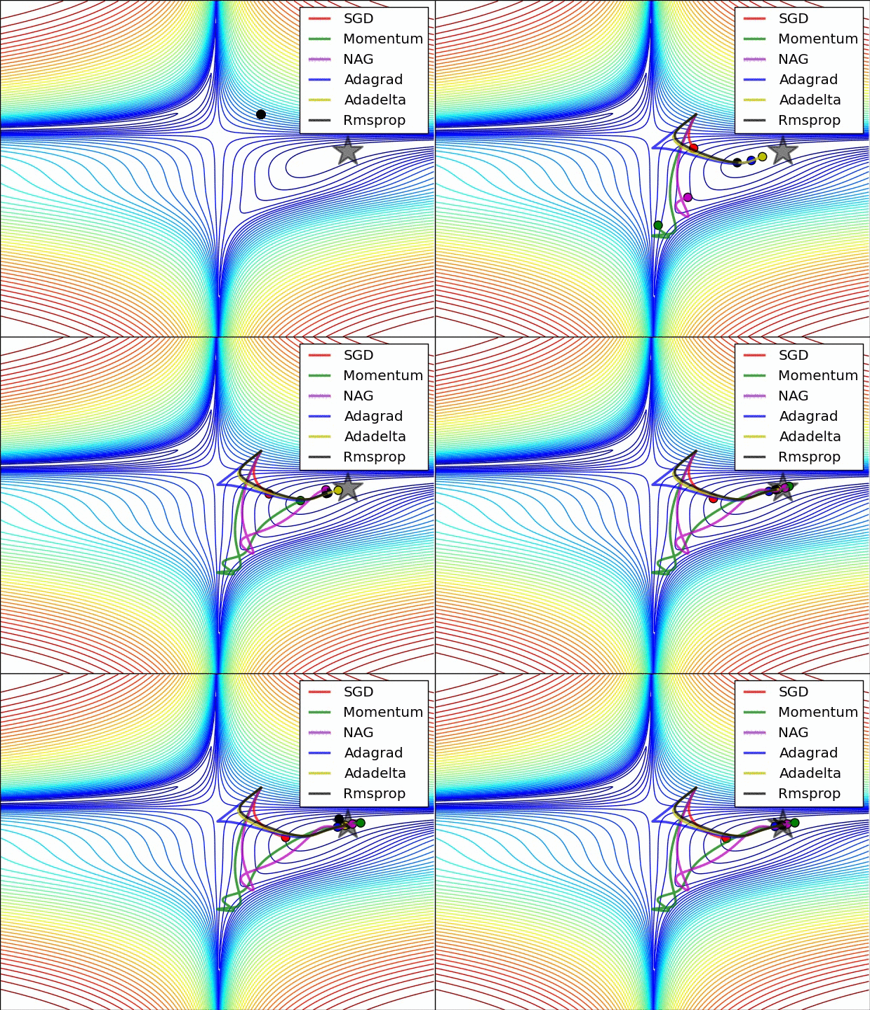
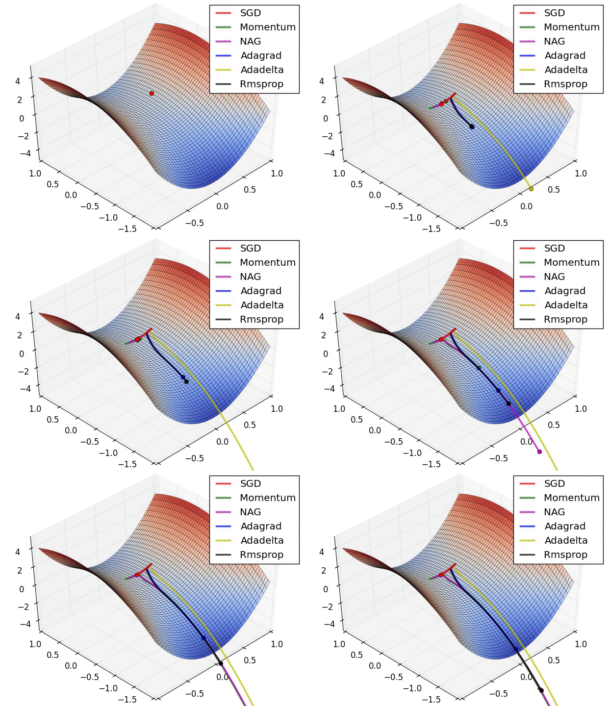
There are some cool visualizations that show how these algorithms behave created by Alec Radford. In the first gif, marked as “Image 5”, we can see the behavior of these algorithms on the contours of the loss surface. Note that here the Beale function was used, and not the MSE. Observe how AdaGrad, Adadelta (variation of AdaGrad), and RMSprop go in the right direction almost immediately. Momentum and NAG are gone off-track in the beginning. NAG quickly corrects its course while Momentum needs some time to pick it up. Also, notice how Stochastic Gradient Descent is slow.
|
|
The second image – “Image 6” explores how these algorithms behave at a saddle point. The saddle point is a point where one dimension has a positive slope, while the other dimension has a negative slope. This is, as we mentioned, a big problem for Stochastic Gradient Descent. Observe how momentum-based optimizers have problems escaping this position. The optimizers that are using adaptive learning rate, however, quickly head down the negative slope.
Conclusion
In this article, we explored optimizers that go beyond Gradient Descent. We covered momentum-based optimizers and the optimizers that adapt the learning rate. We had a chance to implement Momentum Optimizer, Nesterov Accelerated Gradient Optimizer, AdaGrad, RMSProp with Python. Apart from that, we had a chance to take a look at one of the most popular optimizers, which combines all these ideas – Adam.
Thank you for reading!

Nikola M. Zivkovic
CAIO at Rubik's Code
Nikola M. Zivkovic a CAIO at Rubik’s Code and the author of book “Deep Learning for Programmers“. He is loves knowledge sharing, and he is experienced speaker. You can find him speaking at meetups, conferences and as a guest lecturer at the University of Novi Sad.
Rubik’s Code is a boutique data science and software service company with more than 10 years of experience in Machine Learning, Artificial Intelligence & Software development. Check out the services we provide.


Trackbacks/Pingbacks