Double DQN with TensorFlow 2 and TF-Agents

In the previous articles, we covered major reinforcement learning topics. They paved a path to this article which combines those topics under a single umbrella. As a reminder, we talked a lot about the main reinforcement learning elements and how deep learning is used to increase its performance – deep reinforcement learning. This approach to learning is different from the ones that are typical for standard machine learning or deep learning. In these fields supervised learning and unsupervised learning are used, while reinforcement learning relies heavily on the interaction between the learning agent and the environment.

Eager to learn how to build Deep Learning systems using Tensorflow 2 and Python? Get the ebook here!

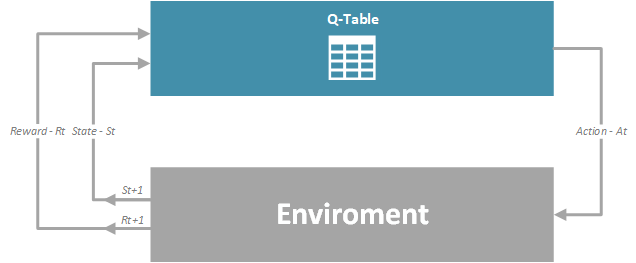
Learning agent performs actions within environment, which puts environment in the certain state. In turn, environment returns reward to the agent. Goal of the learning agent is to maximize the reward. This approach to rewards driven learning, reminds us to Pavlov’s experiments with his dog, which is really interesting. However, let’s not drift far from the subject. In order to mathematically formulate these systems, we use Markov Decision Processes, or MDPs. They are represented as a tuple of four elements:

S – Set of states. At each time step t, the agent gets the environment’s state – St, where St ∈ S.
A – Set of actions that the agent can take.
Pa – Probability that action in some state s will result in the time step t, will result in the state s’ in the time step t+1.
Ra – Or Ra(s, s’), represents expected reward received after going from state s to the state s’, as a result of action a.

MDPs are can be represented using image below:

One approach to solving this problem, and by far the most popular one, presented with MDPs is Q-Learning.

Q-Learning vs Double Q-Learning

We already have multiple articles on our blog about Q-Learning, but let’s have a quick round up. Q-Learning is based on estimation the Q-Value, which is the value of taking action a in state s under policy π. Some consider this as a quality of action a in state s. Larger Q-Value indicates that reward for the learning agent is bigger. The policy in this case defines state–action pairs that visited and updated during the training process. In each epoch of training process, agent updates Q-Values for every state-action combination. That is how it creates a matrix or a table, where for each action and the state we store Q-Value. The process of updating these values is described by the formula:

The important part of the formula above is maxQ(St+1, a). Note the t+1 annotation. This means that current Q-value is based on the Q-value of state in which environment will be after the action is performed. Spooky indeed. How does this work? Well, in the beginning we initialize Q-Values for states St and St+1 to some random values. During the first training iteration we update Q-Value in the state St based on reward and on those random value of Q-Value in the state St+1.

To get it even more clear we can brake down Q-Learning into the steps. It would look something like this:

Initialize all Q-Values in the Q-Table arbitrary, and the Q value of terminal-state to 0:
Q(s, a) = n, ∀s ∈ S, ∀a ∈ A(s)
Q(terminal-state, ·) = 0
Pick the action a, from the set of actions defined for that state A(s) defined by the policy π.
Perform action a
Observe reward R and the next state s’
For all possible actions from the state s’ select the one with the highest Q-Value – a’.
Update value for the state using the formula:
Q(s, a) ← Q(s, a) + α [R + γ*maxQ(s’, a’) − Q(s, a)]
Repeat steps 2-5 for each time step until the terminal state is reached
Repeat steps 2-6 for each episode

However, this crucial part of the formula maxQ(St+1, a) is also the major flaw of Q-Learning. In general, Q-Learning performs poorly in some stochastic environments and max operator is the reason for that. Because of it Q-Learning overestimate Q-Values for certain actions. This means that this algorithm can be tricked that some actions are good even though they provide lower reward in the end. Check out this article for further explanation.

Solution for this problem is Double Q-Learning. It builds on the assumption that instead using one estimator we can use two estimators. In turn, this means that instead of using one Q-Value for each state-action pair, we should use two values – QA and QB. Double Q-Learning focuses on finding action a* that maximizes QA in the next state s’ – (Q(s’, a*) = max Q(s’, a)). Then it uses this action to get the value of second Q-Value – QB(s’, a*). Finally it uses QB(s’, a*) in order to update QA(s, a):

The same process is applied to QB. Here is what it looks like when we brake down Double Q-Learning process into the steps:

Initialize all QA, QB and starting state – s
Repeat
- Pick the action a and based on QA(s, •) and QB(s, •) get r and s’
- Update(A) or Update(B) (pick at random)
- If Update(A)
  - Pick the action a* = argmax QA(s’, a)
  - Update QA
    QA(s, a) ← QA(s, a) + α [R + γQB(s’, a*) − QA(s, a)]
- IfUpdate(B)
  - Pick the action b* = argmax QB(s’, a)
  - Update QB
    QB(s, a) ← QB(s, a) + α [R + γQA(s’, b*) − QB(s, a)]
- s ← s’
Until End

In the previous article, we compared these two algorithms in more details, so make sure to check it out.

DQN and Double DQN

With reticent advances in deep learning, researchers came up with an idea that Q-Learning can be mixed with neural networks. That is how the deep reinforcement learning, or Deep Q-Learning to be precise, were born. Instead of using Q-Tables, Deep Q-Learning or DQN is using two neural networks. In this architecture, networks are feed forward neural networks which are utilized for predicting the best Q-Value. Because input data is not provided beforehand, the agent has to store previous experiences in a local memory called experience reply. This information is then used as input data.

It is important to notice that DQNs don’t use supervised learning like majority of neural networks. The reason for that is lack of labels (or expected output). These are not provided to the learning agent beforehand, i.e. learning agent has to figure them out on its own. Because every Q-Value depends on the policy, target (expected output) is continuously changing with each iteration. This is the main reason why this type of learning agent doesn’t have just one neural network, but two of them. The first network, which is refereed to as Q-Network is calculating Q-Value in the state St. The second network, refereed to as Target Network is calculating Q-Value in the state St+1.

Speaking more formally, given the current state St, the Q-Network retrieves the action-values Q(St,a). At the same time the Target Network uses the next state St+1 to calculate Q(St+1, a) for the Temporal Difference target. In order to stabilize this training of two networks, on each N-th iteration parameters of the Q-Network are copied over to the Target Network. Mathematically, a deep Q network (DQN) is represented as a neural network that for a given state s outputs a vector of action values Q(s, · ; θ), where θ are the parameters of the network. The Target Network, with parameters θ −, is the same as the Q-Network, but its parameters are copied every τ steps from the online network, so that then θ − t = θt. The target itself used by DQN is then defined like this:

A while back we implemented this process using Python and Tensorflow 2. You can check out that implementation here. Also, we used TF-Agents for implementation as well and you can find that here.

The problem with DQN is essentially the same as with vanilla Q-Learning, it overestimates Q-Values. So, this concept is extended with the knowledge from the Double Q-Learning and Double DQN was born. It represents minimal possible change to DQN. Personally, i think it is rather elegant how the author was able to get most of the benefits of Double Q-learning, while keeping the DQN algorithm the same. The core of the Double Q-learning is that it reduces Q-Value overestimations by splinting max operator into action selection and action evaluation. This is where target network in DQN algorithm played a major role. Meaning, no additional networks are added to the system, but evaluation of the policy of the Q-Network is done by using the Target Network to estimate its value. So, only the target is changes in Double DQN:

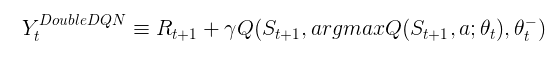
To sum it up, weights of the second network are replaced with the weights of the target network for the evaluation of the policy. Target Network is still updated periodically, by copying parameters from Q-Network.

Implementation

Prerequisites

This article contains two implementations of Double DQN. Both are done with Python 3.7 and using the Open AI Gym. First implementation uses TensorFlow 2 and the second one uses TF-Agents. Make sure you have these installed on your environment:

Python 3.7
TensorFlow 2.1.0
TF-Agents
Open AI Gym

If you need to learn more about TensorFlow 2, check out this guide and if you need to get familiar with TF-Agents, we recommend this guide.

In this article we use famous CartPole-v0 enviroment:

A pole is attached to a cart which moves along a track in this environment. The whole structure is controlled by applying a force of +1 or -1 to the cart and moving it left or right. The pole is in upright position in the beginning, and the goal is to prevent it from falling. For every timestamp in which pole doesn’t fall a reward of +1 is provided. The complete episode ends when the pole is more than 15 degrees from vertical, or the cart moves more than 2.4 units from the center.

TensorFlow 2 Implementation

Let’s kick off this implementation with modules that we need to import:

import gym
import tensorflow as tf
from collections import deque

import random
import numpy as np
import math

from tensorflow.keras import Model, Sequential
from tensorflow.keras.layers import Dense, Conv2D, Flatten, Input
from tensorflow.keras.optimizers import Adam
from tensorflow.keras.losses import Huber
from tensorflow.keras.initializers import he_normal
from tensorflow.keras.callbacks import History

Apart from that, here are some of the global constants we need to define.

MAX_EPSILON = 1
MIN_EPSILON = 0.01

GAMMA = 0.95
LAMBDA = 0.0005
TAU = 0.08

BATCH_SIZE = 32
REWARD_STD = 1.0

MAX_EPSILON and MIN_EPSILON are used to control exploration to exploration ratio. While others are used during training process. REWARD_STD has special meaning, which we will check out later on. Now, we need to load the environment.

enviroment = gym.make("CartPole-v0")

NUM_STATES = 4
NUM_ACTIONS = enviroment.action_space.n

We also defined number of states and actions that are available in this environment. Next thing we need to take care of is experience reply. This is a buffer that holds information that are used during training process. Implementation is looks like this:

class ExpirienceReplay:
    def __init__(self, maxlen = 2000):
        self._buffer = deque(maxlen=maxlen)
    
    def store(self, state, action, reward, next_state, terminated):
        self._buffer.append((state, action, reward, next_state, terminated))
              
    def get_batch(self, batch_size):
        if no_samples > len(self._samples):
            return random.sample(self._buffer, len(self._samples))
        else:
            return random.sample(self._buffer, batch_size)
        
    def get_arrays_from_batch(self, batch):
        states = np.array([x[0] for x in batch])
        actions = np.array([x[1] for x in batch])
        rewards = np.array([x[2] for x in batch])
        next_states = np.array([(np.zeros(NUM_STATES) if x[3] is None else x[3]) 
                                for x in batch])
        
        return states, actions, rewards, next_states
        
    @property
    def buffer_size(self):
        return len(self._buffer)

Note that this class does minor pre-processing as well. That happens in the function get_arrays_from_batch. This method returns arrays of states, actions, rewards and next states deconstructed from the batch. Ok, to the fun part. Here is the implantation of the Double DQN Agent:

class DDQNAgent:
    def __init__(self, expirience_replay, state_size, actions_size, optimizer):
        
        # Initialize atributes
        self._state_size = state_size
        self._action_size = actions_size
        self._optimizer = optimizer
        
        self.expirience_replay = expirience_replay
        
        # Initialize discount and exploration rate
        self.epsilon = MAX_EPSILON
        
        # Build networks
        self.primary_network = self._build_network()
        self.primary_network.compile(loss='mse', optimizer=self._optimizer)

        self.target_network = self._build_network()   
   
    def _build_network(self):
        network = Sequential()
        network.add(Dense(30, activation='relu', kernel_initializer=he_normal()))
        network.add(Dense(30, activation='relu', kernel_initializer=he_normal()))
        network.add(Dense(self._action_size))
        
        return network
    
    def align_epsilon(self, step):
        self.epsilon = MIN_EPSILON + (MAX_EPSILON - MIN_EPSILON) * math.exp(-LAMBDA * step)
    
    def align_target_network(self):
        for t, e in zip(self.target_network.trainable_variables, 
                    self.primary_network.trainable_variables): t.assign(t * (1 - TAU) + e * TAU)
    
    def act(self, state):
        if np.random.rand() < self.epsilon:
            return np.random.randint(0, self._action_size - 1)
        else:
            q_values = self.primary_network(state.reshape(1, -1))
            return np.argmax(q_values)
    
    def store(self, state, action, reward, next_state, terminated):
        self.expirience_replay.store(state, action, reward, next_state, terminated)
    
    def train(self, batch_size):
        if self.expirience_replay.buffer_size < BATCH_SIZE * 3:
            return 0
        
        batch = self.expirience_replay.get_batch(batch_size)
        states, actions, rewards, next_states = expirience_replay.get_arrays_from_batch(batch)
        
        # Predict Q(s,a) and Q(s',a') given the batch of states
        q_values_state = self.primary_network(states).numpy()
        q_values_next_state = self.primary_network(next_states).numpy()
        
        # Copy the q_values_state into the target
        target = q_values_state
        updates = np.zeros(rewards.shape)
                
        valid_indexes = np.array(next_states).sum(axis=1) != 0
        batch_indexes = np.arange(BATCH_SIZE)

        action = np.argmax(q_values_next_state, axis=1)
        q_next_state_target = self.target_network(next_states)
        updates[valid_indexes] = rewards[valid_indexes] + GAMMA * 
                  q_next_state_target.numpy()[batch_indexes[valid_indexes], action[valid_indexes]]
        
        target[batch_indexes, actions] = updates
        loss = self.primary_network.train_on_batch(states, target)

        # update target network parameters slowly from primary network
        self.align_target_network()
        
        return loss

In the constructor of DDQNAgent class, apart from initializing fields, we use internal _build_network method to build two networks. Note that we compile only the Q-Network or the primary network. Also, note the rich API this class exposes:

align_epsilon – This method is used to update the epsilon value. This value represents exploration to exploration ratio. The goal is to explore more actions in the begging of training, but slowly switch to exploiting learned actions later on.
align_target_network – We use this method to slowly copy over parameters from Q-Network to Target Network.
act – This important function returns action that should be taken in the defined state taking into epsilon into consideration.
store – Stores values into experience replay.
train – Performs single training iteration.

Let’s observe train method more closely:

def train(self, batch_size):
        if self.expirience_replay.buffer_size < BATCH_SIZE * 3:
            return 0
        
        batch = self.expirience_replay.get_batch(batch_size)
        states, actions, rewards, next_states = expirience_replay.get_arrays_from_batch(batch)
        
        # Predict Q(s,a) and Q(s',a') given the batch of states
        q_values_state = self.primary_network(states).numpy()
        q_values_next_state = self.primary_network(next_states).numpy()
        
        # Initialize target
        target = q_values_state
        updates = np.zeros(rewards.shape)
                
        valid_indexes = np.array(next_states).sum(axis=1) != 0
        batch_indexes = np.arange(BATCH_SIZE)

        action = np.argmax(q_values_next_state, axis=1)
        q_next_state_target = self.target_network(next_states)
        updates[valid_indexes] = rewards[valid_indexes] + GAMMA * 
              q_next_state_target.numpy()[batch_indexes[valid_indexes], action[valid_indexes]]
        
        target[batch_indexes, actions] = updates
        loss = self.primary_network.train_on_batch(states, target)

        # Slowly update target network parameters from primary network
        self.align_target_network()
        
        return loss

First, we make sure that we have enough data in experience replay buffer. If we have enough data, we pick up batch of data and split it into arrays. Then we get Q(s,a) and Q(s’,a’) using Q-Network or primary network. After that, we pick the action and use the Train Network to predict Q(s’,a’). We generate the updates for the target and use it to train Q-Network. Finally, we copy over values from the Q-Network to the Target Network.

However, this train function is just part of the whole training process, so we define one class above that that combines agent and environment, and drives the whole process – AgentTrainer. Here is what it looks like:

class AgentTrainer():
    def __init__(self, agent, enviroment):
        self.agent = agent
        self.enviroment = enviroment
        
    def _take_action(self, action):
        next_state, reward, terminated, _ = self.enviroment.step(action) 
        next_state = next_state if not terminated else None
        reward = np.random.normal(1.0, REWARD_STD)
        return next_state, reward, terminated
    
    def _print_epoch_values(self, episode, total_epoch_reward, average_loss):
        print("**********************************")
        print(f"Episode: {episode} - Reward: {total_epoch_reward} - Average Loss: {average_loss:.3f}")
    
    def train(self, num_of_episodes = 1000):
        total_timesteps = 0  
        
        for episode in range(0, num_of_episodes):

            # Reset the enviroment
            state = self.enviroment.reset()

            # Initialize variables
            average_loss_per_episode = []
            average_loss = 0
            total_epoch_reward = 0

            terminated = False

            while not terminated:

                # Run Action
                action = agent.act(state)

                # Take action    
                next_state, reward, terminated = self._take_action(action)
                agent.store(state, action, reward, next_state, terminated)
                
                loss = agent.train(BATCH_SIZE)
                average_loss += loss

                state = next_state
                agent.align_epsilon(total_timesteps)
                total_timesteps += 1

                if terminated:
                    average_loss /= total_epoch_reward
                    average_loss_per_episode.append(average_loss)
                    self._print_epoch_values(episode, total_epoch_reward, average_loss)
                
                # Real Reward is always 1 for Cart-Pole enviroment
                total_epoch_reward +=1

This class has several methods. First internal method _take_action is rather interesting. In this method, we use environment that is passed in the constructor to perform defined action. Now, the interesting part is that we change nature of the Cart-Pole environment by changing reward it returns. To be more precise, this environment is deterministic, but we want it to be stochastic because Double DQN performs better in that kind of environments. Since the reward is always +1, we replaced it with a sample from normal distribution. That is where we use REWARD_STD that we mentioned previously.

In the train method of AgentTrainer we perform run the training process for the defined number of epochs. The process follows Double DQN algorithm steps. For each epoch, we pick an action and execute it in the environment. This gives us necessary information for training the agent and its neural networks, after which we get loss. Finally, we calculate average loss for each epoch. Alright, when we put it all together it looks something like this:

optimizer = Adam()
expirience_replay = ExpirienceReplay(50000)
agent = DDQNAgent(expirience_replay, NUM_STATES, NUM_ACTIONS, optimizer)
agent_trainer = AgentTrainer(agent, enviroment)
agent_trainer.train()

And here is the output:

*******************************
Episode: 0 - Reward: 13 - Average Loss: 2.153
 ******************************* 
Episode: 1 - Reward: 9 - Average Loss: 1.088
 ******************************* 
Episode: 2 - Reward: 12 - Average Loss: 1.575
 ******************************* 
Episode: 3 - Reward: 14 - Average Loss: 0.973
 ******************************* 
Episode: 4 - Reward: 23 - Average Loss: 1.451
 ******************************* 
Episode: 5 - Reward: 29 - Average Loss: 1.463
 ******************************* 
Episode: 6 - Reward: 28 - Average Loss: 1.265
 ******************************* 
Episode: 7 - Reward: 20 - Average Loss: 1.520
 ******************************* 
Episode: 8 - Reward: 10 - Average Loss: 1.201
 ******************************* 
Episode: 9 - Reward: 25 - Average Loss: 0.976
 ******************************* 
Episode: 10 - Reward: 33 - Average Loss: 1.408
...

TF-Agent Implementation

TensorFlow implementation of this process was not complicated, but it is always easier to have some precooked classes that you can use. For reinforcement learning we can use TF-Agents. In one of the previous articles, we saw how one can use this tool to build DQN system. Let’s see how we can do the same and build Double DQN with TF-Agents. Again, first we import modules and define constants:

import base64
import imageio
import matplotlib
import matplotlib.pyplot as plt

import tensorflow as tf

from tf_agents.agents.dqn.dqn_agent import DqnAgent, DdqnAgent
from tf_agents.networks.q_network import QNetwork

from tf_agents.environments import suite_gym
from tf_agents.environments import tf_py_environment

from tf_agents.policies.random_tf_policy import RandomTFPolicy
from tf_agents.replay_buffers.tf_uniform_replay_buffer import TFUniformReplayBuffer
from tf_agents.trajectories import trajectory
from tf_agents.utils import common

# Globals
NUMBER_EPOSODES = 20000
COLLECTION_STEPS = 1
BATCH_SIZE = 64
EVAL_EPISODES = 10
EVAL_INTERVAL = 1000

One of the cool things about TF-Agents is that it provides us with easy way to load environments without installing additional modules. That way we only use this ecosystem and don’t have to worry about missing modules. Here is how we load the environment:

train_env = suite_gym.load('CartPole-v0')
evaluation_env = suite_gym.load('CartPole-v0')

print('Observation Spec:')
print(train_env.time_step_spec().observation)

print('Reward Spec:')
print(train_env.time_step_spec().reward)

print('Action Spec:')
print(train_env.action_spec())

train_env = tf_py_environment.TFPyEnvironment(train_env)
evaluation_env = tf_py_environment.TFPyEnvironment(evaluation_env)

Because we want to run DQN and Double DQN together for comparison, we create two Q-Networks. Underneath, this creates Target Networks and takes care of the maintenance of both networks.

hidden_layers = (100,)

dqn_network = QNetwork(
    train_env.observation_spec(),
    train_env.action_spec(),
    fc_layer_params=hidden_layers)

ddqn_network = QNetwork(
    train_env.observation_spec(),
    train_env.action_spec(),
    fc_layer_params=hidden_layers)

Once that is done, we can create two agents. First one is used for DQN and the other one for Double DQN. TF-Agents provides classes for this as well:

counter = tf.Variable(0)

dqn_agent = DqnAgent(
    train_env.time_step_spec(),
    train_env.action_spec(),
    q_network = dqn_network,
    optimizer = tf.compat.v1.train.AdamOptimizer(learning_rate=1e-3),
    td_errors_loss_fn = common.element_wise_squared_loss,
    train_step_counter = counter)

ddqn_agent = DdqnAgent(
    train_env.time_step_spec(),
    train_env.action_spec(),
    q_network = ddqn_network,
    optimizer = tf.compat.v1.train.AdamOptimizer(learning_rate=1e-3),
    td_errors_loss_fn = common.element_wise_squared_loss,
    train_step_counter = counter)

dqn_agent.initialize()
ddqn_agent.initialize()

These objects are initialized with information about training environment, object of the QNetwork and the optimizer. In the end, we must call initialize method on them. We implement one more function on top of this – get_average_return. This method calculates how much reword has agent gained on average.

def get_average_reward(environment, policy, episodes=10):

    total_reward = 0.0

    for _ in range(episodes):
        time_step = environment.reset()
        episode_reward = 0.0

    while not time_step.is_last():
        action_step = policy.action(time_step)
        time_step = environment.step(action_step.action)
        episode_reward += time_step.reward
    
    total_reward += episode_reward
    avg_reward = total_reward / episodes
    
    return avg_reward.numpy()[0]

So far, so good. Now, we build the final part of the system – experience replay.

class ExperienceReplay(object):
    def __init__(self, agent, enviroment):
        self._replay_buffer = TFUniformReplayBuffer(
            data_spec=agent.collect_data_spec,
            batch_size=enviroment.batch_size,
            max_length=50000)
        
        self._random_policy = RandomTFPolicy(train_env.time_step_spec(),
                                                enviroment.action_spec())
        
        self._fill_buffer(train_env, self._random_policy, steps=100)
        
        self.dataset = self._replay_buffer.as_dataset(
            num_parallel_calls=3, 
            sample_batch_size=BATCH_SIZE, 
            num_steps=2).prefetch(3)

        self.iterator = iter(self.dataset)
    
    def _fill_buffer(self, enviroment, policy, steps):
        for _ in range(steps):
            self.timestamp_data(enviroment, policy)
            
    def timestamp_data(self, environment, policy):
        time_step = environment.current_time_step()
        action_step = policy.action(time_step)
        next_time_step = environment.step(action_step.action)
        timestamp_trajectory = trajectory.from_transition(time_step, action_step, next_time_step)

        self._replay_buffer.add_batch(timestamp_trajectory)

First, we initialize replay buffer in the constructor of the class. This is an object of the class TFUniformReplayBuffer. If your agent performs poorly, you can change values of batch size and length of the buffer. Apart from that, we create an instance of RandomTFPolicy. This object fills buffer with initial values. This process is initiated by the method _fill_buffer. This method in calls timestamp_data method for each state of the environment, which in turn forms trajectory from the current state and the action defined by policy. This trajectory is tuple of state, action and next timestamp, and it is stored in the the buffer. Final step of the constructor is to create an iterable tf.data.Dataset pipeline which feeds data to the agent.

Finally, we can combine all these elements within train function:

def train(agent):
    experience_replay = ExperienceReplay(agent, train_env)

    agent.train_step_counter.assign(0)

    avg_reward = get_average_reward(evaluation_env, agent.policy, EVAL_EPISODES)
    rewards = [avg_reward]

    for _ in range(NUMBER_EPOSODES):

        for _ in range(COLLECTION_STEPS):
            experience_replay.timestamp_data(train_env, agent.collect_policy)

        experience, info = next(experience_replay.iterator)
        train_loss = agent.train(experience).loss

        if agent.train_step_counter.numpy() % EVAL_INTERVAL == 0:
            avg_reward = get_average_reward(evaluation_env, agent.policy, EVAL_EPISODES)
            print('Episode {0} - Average reward = {1}, Loss = {2}.'.format(
					agent.train_step_counter.numpy(), avg_reward, train_loss))
            rewards.append(avg_reward)
            
    return rewards

print("**********************************")
print("Training DQN")
print("**********************************")
dqn_reward = train(dqn_agent)

print("**********************************")
print("Training DDQN")
print("**********************************")
ddqn_reward = train(ddqn_agent)

When we run the function the output looks like this:

********************************** 
Training DQN 
********************************** 
Episode 1000 - Average reward = 2.700000047683716, Loss = 95.45304870605469. 
Episode 2000 - Average reward = 2.299999952316284, Loss = 41.39720916748047. 
Episode 3000 - Average reward = 3.799999952316284, Loss = 34.7718620300293. 
Episode 4000 - Average reward = 5.599999904632568, Loss = 123.10957336425781. 
Episode 5000 - Average reward = 8.100000381469727, Loss = 171.66470336914062. 
Episode 6000 - Average reward = 15.899999618530273, Loss = 209.91107177734375. 
Episode 7000 - Average reward = 20.0, Loss = 130.32858276367188. 
Episode 8000 - Average reward = 20.0, Loss = 14.633146286010742. 
Episode 9000 - Average reward = 20.0, Loss = 188.2078857421875. 
Episode 10000 - Average reward = 20.0, Loss = 31.698490142822266. 
Episode 11000 - Average reward = 20.0, Loss = 306.1351013183594. 
... 
**********************************  
Training DDQN  
**********************************  
Episode 1000 - Average reward = 1.0, Loss = 0.6193162202835083.  
Episode 2000 - Average reward = 5.699999809265137, Loss = 6.596433639526367.  
Episode 3000 - Average reward = 7.699999809265137, Loss = 16.949800491333008. 
Episode 4000 - Average reward = 6.699999809265137, Loss = 19.932825088500977.  
Episode 5000 - Average reward = 20.0, Loss = 4.6859331130981445.  
Episode 6000 - Average reward = 20.0, Loss = 5.8436055183410645.  
Episode 7000 - Average reward = 20.0, Loss = 44.722599029541016.  
Episode 8000 - Average reward = 20.0, Loss = 98.11009979248047.  
Episode 9000 - Average reward = 20.0, Loss = 11.548649787902832.  
Episode 10000 - Average reward = 20.0, Loss = 147.0045623779297.  
Episode 11000 - Average reward = 14.5, Loss = 321.64013671875. 
 ...

In the end, we can plot average reward for both agents:

episodes = range(0, NUMBER_EPOSODES + 1, EVAL_INTERVAL)
plt.plot(episodes, dqn_reward, label = 'DQN Rewards')
plt.plot(episodes, ddqn_reward, label = 'DDQN Rewards')
plt.legend()
plt.ylabel('Average reward')
plt.xlabel('Epoisodes')
plt.ylim(top=50)

We can see that Double DQN creates better policy quicker and gets to the stable state.

Conclusion

In this article, we had a chance to see how we can enrich out DQN algorithm using concepts from Double Q-Learning and create Double DQN. Apart from that we had a chance to implement this algorithm using both TensorFlow and TF-Agents.

Thank you for reading!

Nikola M. Zivkovic

CAIO at Rubik's Code

Nikola M. Zivkovic a CAIO at Rubik’s Code and the author of book “Deep Learning for Programmers“. He is loves knowledge sharing, and he is experienced speaker. You can find him speaking at meetups, conferences and as a guest lecturer at the University of Novi Sad.

Rubik’s Code is a boutique data science and software service company with more than 10 years of experience in Machine Learning, Artificial Intelligence & Software development. Check out the services we provide.