Top 3 Artificial Intelligence Research Papers – July 2020

Every month, we decipher three research papers from the fields of machine learning, deep learning and artificial intelligence, which left an impact on us in the previous month. Apart from that, at the end of the article, we add links to other papers that we have found interesting but were not in our focus that month. So, you can check those as well. Here are the links from the previous months:

• January
• February
• March
• April
• May
• June 

In general, we try to present papers that are going to leave a big impact on the future of machine learning and deep learning. We believe that these proposals are going to change the way we do our jobs and push the whole field forward. Have fun!

PP-YOLO: An Effective and Efficient Implementation of Object Detector

YOLOv3 became a sort of industry standard when it comes to object detection due to its excellent effectiveness and efficiency. Many of our clients are using this architecture for this important computer vision task. A couple of months ago, the YOLOv4 paper was published. Unlike previous versions of YOLO, this paper doesn’t make big changes architecturally speaking, but focuses on various strategies such as a bag of freebies and bag of specials on the basis of YOLOv3. Improving performances of YOLOv3 seems to be the main goal, not it’s redefinition.

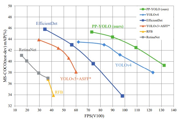
This paper focuses on that as well. In fact, it is not proposing some novel approach or architecture, but it provides effective guidelines that leed to better performance but don’t affect the accuracy. It provides valuable tips and tricks for developers. The model that the authors proposed is called PP-YOLO because it majority of tricks are based on PaddlePaddle. The final result improves the mAP on COCO from 43.5% to 45.2% at a speed faster than YOLOv4, so let’s check to see what these tricks are all about.

The proposals from this paper cannot be directly applied to the network structure of YOLOv3 and small modifications are required. So, let’s go through the YOLOv3 structure before we dive into tips and tricks this paper proposes. YOLOv3 belongs to a one-stage object detector which is composed of backbone network (usually ResNet), a detection neck (usually FPN), and a detection head for object classification and localization.

As a backbone YOLOv3 uses DarkNet-53. The authors replace the backbone with ResNet-50-vd-dcn. This network is essentially ResNet-50-vd with the addition of deformable convolutional layers (DCN), ie. 3 × 3 convolution layers in the last stage are replaced with DCNs. Some minor changes are performed in the FPN network that is used as a detection neck. As a detection head, YOLOv3 uses a pretty simple Convolutional Neural Network that has one 3×3 convolutional layer followed by an 1×1 convolutional layer. Below you can find the complete architecture along with the injection points of PP-YOLO, ie. changes made by this paper.

Ok, let’s go through the list of tips proposed in this article. Note that some of these tricks can be applied to YOLOv3 directly:

• Larger Batch Size – Increase training batch size from 64 to 192, and adjust the training schedule and learning rate accordingly.
• Exponential Moving Average (EMA) – During the training process, maintaining moving averages of the trained parameters can be useful since evaluations that use averaged parameters sometimes produce significantly better results. Authors thus suggest maintaining shadow parameter (WEMA) for each parameter W, which is used for evaluation: WEMA = λWEMA + (1 − λ)W
• DropBlock on FPN – Use dropout only on FPN, not on the whole YOLOv3 network.
• IoU Loss – YOLOv4 replaces the L1-loss, which is used in YOLOv3 for bounding box regression with IoU loss. Unlike that approach, authors just add another branch to calculate IoU loss.
• IoU Aware – Since in YOLOv3 detection confidence is calculated by multiplying classification probabilities and objectness score, localization accuracy is not taken into consideration. In order to solve this problem, another IoU branch is added to measure the accuracy of localization.
• Grid Sensitive – This trick is introduced by YOLOv4. Since it is difficult to predict centers of bounding boxes located on the grid boundary, formulas for calculating coordinates of these centers are modified:
  x = s · (gx + 1.05 · σ(px) − (1.05 − 1)/2)
  y = s · (gy + 1.05 · σ(py) − (1.05 − 1)/2)
• Matrix NMS – Matrix NMS is technically Soft-NMS done in parallel. That is why it is faster than traditional NMS.
• CoordConv – The 1×1 convolution layer in FPN and the first convolution layer in the detection head are replaced with CoordConv layers. These layers allow networks to learn either complete translation invariance or varying degrees of translation dependence. Essentially it adds extra coordinate channels and thus provides convolution access to its own input coordinates.
• SPP – Unlike YOLOv4 SPP is only applied on the top feature map. On the image above it is marked with ”star”.
• Better Pretrain Model – This is sort of obvious, but if you use a model that was trained better for the backbone the results will be better.

This approach proves to be really good since PP-YOLO is faster (FPS) and more accurate(COCO mAP) than EfficientDet and YOLOv4. The results can be seen in the graph above.

Learning to Match Distributions for Domain Adaptation

This paper addresses a big problem in our industry. We usually train our predictive models on the training dataset and then test it on the testing dataset. There is always a drop in the performance between training data and testing data. This we accept as normal because we know that these datasets don’t have the same distribution. The problem is that our approach generally assumes that. We try to minimize that gap by getting more data, but that can be expensive.

To ensure consistent performance of predictive models domain adaptation is performed. The main aim of this process is to match the cross-domain joint distributions. However, this is not always possible, plus in unsupervised we don’t have a target domain. Theoretically, matching the joint distributions by matching the marginal and conditional distributions should do the trick and solutions presented thus far are using this approach. Still, applying it to new applications remains problematic.

The authors of this paper focused on making data-driven solutions that is inspired by deep learning. As you know, the main advantage of deep learning over traditional machine learning is that it can extract features from the data, so the authors apply a similar principle to the automatic distribution matching strategy. Their solution Learning to Match (L2M) is a framework that is able to combine the deep features and human-crafted features. In essence, it is having GAN-ish architecture and it is composed of two networks meta-network (feed-forward network used as approximator) and feature generator.

The complete methodology of the proposed solution can be broken down into several steps and utilizes architecture from the image above. Architecture is composed of four parts: feature extractor, label classifier, meta-network, and matching feature generator. Feature Extractor is a CNN network that is in charge of extracting features from the input domain. The label classifier minimizes the prediction loss on the labeled source domain. Meta network is the feed-forward neural network used to match cross-domain distributions and learns distribution matching functions. Finally, a feature generator is used to generate useful inputs to the meta-network.

As mentioned, there are two kinds of matching features. The first kind, the task-independent features are general. They can be automatically extracted by the feature extractor. The second kind, Human-designed features are the pre-defined features such as MMD or adversarial game. They are represented with box D in the image above.

If L2M is used for unsupervised learning or we are missing the target domain, so the optimization is performed by generating meta-data in a self-supervised manner. This meta-data is then used to update distribution matching loss. In each iteration, we randomly sample n instances for each class with high prediction scores. This is done feature extractor and the results are stored as the ground truth of the meta-data. This way the pseudo labels of the meta-data are getting better since we utilize data with the highest prediction probabilities.

The results are amazing. Experiments on public datasets substantiate the superiority of L2M over state-of-the-art approaches on DA and image generation tasks. The notable result can be seen in the COVID-19 X-ray image adaptation experiment, which is the representation of a highly imbalanced task, where this approach outperforms existing methods.

Generative Pretraining from Pixels

While unsupervised pre-training has its roots in the visual tasks, today it is predominant in Natural Language Processing. This is really interesting, because even in BERT, the Transformer-like architecture used in NLP, the prediction of corrupted inputs, is similar to that of the Denoising Autoencoder which was developed for images. Authors decided to bring back those ideas into the domain where it originated from, and they examine whether models similar to the ones used in NLP can be used images too. They also rely on recent advances of self-supervised methods.

Just like in language tasks, their approach consists of two phases: pre-training and fine-tuning. Also, in order to measure representation quality, they take into consideration both auto-regressive and BERT objectives. In general, there are two ways we can observe this two-stage approach in the context of the image tasks. One way is to observe a pre-training as an initializer or as a regularizer. In order to measure representation quality, fine-tuning is then adapted for image classification, ie. classification head is added to the model which is used for optimization. The other way to observe a two-way approach in the context of this domain is to observe the pre-training phase as a feature extractor. More about how objectives are modified for the purpose of the images you can see in the paper.

The architecture has standard Transformer architecture. The input sequence of tokens is pushed to the transformer decoder which creates a d-dimensional embedding for each position. Each transformer decoder block uses Generative Pretraining from Pixels (GPT) formula on intermediate embeddings:

As you can see, layer norms are used before both attention and feed-forward network operations, and all operations lie on the residual paths. The only mixing of the sequences happens in the attention operation. It is important to note that spatial relationships between positions must be learned during training time. Also, note that after the final transformer layer the layer norm is applied once again. That is how this architecture learns a projection from nL to logits parameterizing the conditional distributions at each sequence element. During fine-tuning average pool nL across the sequence dimension is calculated:

Then projection from fL to class logits is learned. Finally, these projections are used to minimize a cross-entropy loss LCLF. The largest model produced this way iGPT-XL, contains 60 layers and uses an embedding size 3072. It has 6.8B parameters.

The results are really interesting. In the graph above the compared results are shown. Blue bars represent linear probe accuracy and orange bars display finetune accuracy. We can see that Auto-regressive models produce better features than BERT models after pre-training. However, BERT models catch up after fine-tuning.

Other Amazing Papers from this Month

• BabyAI 1.1
• On the Convergence of Tsetlin Machines for the IDENTITY- and NOT Operators
• Regularizing Deep Networks with Semantic Data Augmentation
• Closed-Form Factorization of Latent Semantics in GANs
• SegFix: Model-Agnostic Boundary Refinement for Segmentation

Conclusion

In this article, we had a chance to real about three really cool papers that, as we see it, are going to change the way we perform our jobs. Did you have any favorites this month? Let us know.

Thank you for reading!